매일매일 딥러닝

• paper) https://arxiv.org/pdf/2006.11239.pdf (UC Berkeley)
• code) https://github.com/hojonathanho/diffusion
• original diffusion model paper) https://arxiv.org/pdf/1503.03585.pdf

•  요약
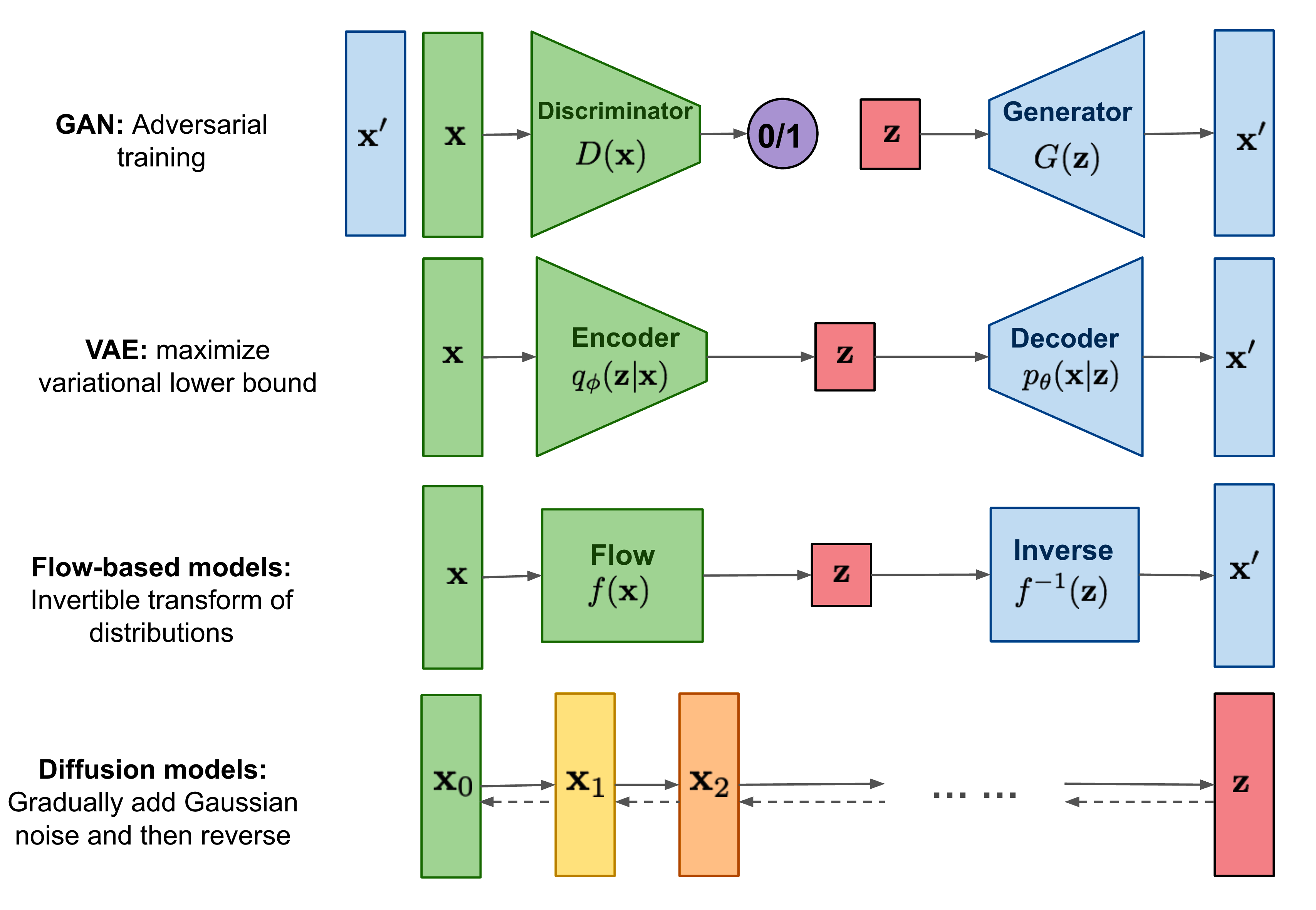
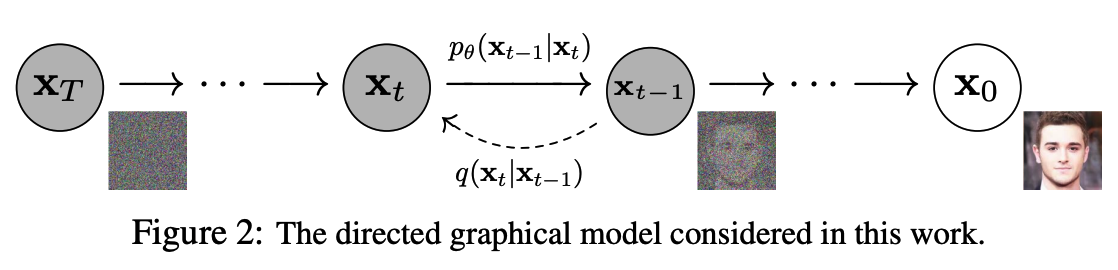
  1. forward diffusion process $q(\mathbf{x}t|\mathbf{x}{t-1})$: noise를 점점 증가 시켜 가면서 학습 데이터를 특정한(Gaussian) noise distribution으로 변환
  2. reverse generative process $p_\theta(\mathbf{x}_{t-1}|\mathbf{x}_t)$: noise distribution으로부터 학습 데이터를 복원(=denoising)하는 것을 학습단 위과정을 Markov Chain으로 표현.
• 왜 잘될까?
  • 기존의 AutoEncoder와 같은 모델의 경우 Encoder 부분에서 어느 정도로 data가 encoding이 될지 알 수 없고 조절할 수 없었지만 Diffusion 모델의 경우 각 time step 마다 약간의 noise가 추가되고 reverse할 때 그 지정된 만큼(?), 종류(?)의 noise를 복원해내면 되기 때문이지 않을까..(마치 작은 tasks로 쪼개서 문제를 해결해나가듯)

1. Introduction

diffusion probabilistic model은 샘플에 매칭되는 데이터를 생성하기위해 variational inference를 사용하여 훈련된 parameterized Markov chain이다.

** Variational Inference 참고

(기계학습, Machine Learning) Week 1 Variational Inference | Lecture 1

** Markov chain: 마르코프 성질을 가진 이산 확률과정을 뜻합니다. (from wiki)

마르코프 성질은 과거와 현재 상태가 주어졌을 때의 미래 상태의 조건부 확률 분포가 과거 상태와는 독립적으로 현재 상태에 의해서만 결정된다는 것을 뜻한다.

이 Transition은 signal이 파괴될때까지(?= $x_0$까지) 샘플링의 반대반향으로 데이터에 노이즈를 점진적으로 추가하는 Markov chain의 diffusion process를 reverse하도록 학습된다.

diffusion이 적은 양의 Gaussian noise로 구성된 경우 샘플링 프로세스의 전환도 조건부 Gaussian으로 설정하면 충분하기때문에 간단한 neural network parameterization이 가능하다.

또한 diffusion model의 특정 parameterization은 훈련 중 multiple noise level에서 denoising score matching하는 것과 샘플링 중 Langevin dynamics 문제를 푸는 것과 동등하다는 것을 발견했다.

** Langevin dynamics (https://yang-song.github.io/blog/2021/score/)

Langevin dynamics provides an MCMC procedure to sample from a distribution $p(x)$ using only its score function $\nabla_\mathbf{x}\text{log} p(\mathbf{x})$.

$s_\theta \approx \nabla_\mathbf{x}\text{log} p(\mathbf{x})$

[Using Langevin dynamics to sample from a mixture of two Gaussians.]

이 논문에서는 diffusion model의 샘플링 프로세스가 autoregressive 모델로 일반화가 가능하다는 것과 autoregressive의 decoding과 유사한 일종의 점진적 decoding이라는 것을 보여준다.

** autoregressive decoder: 과거의 자기 자신을 사용하여 현재의 자신을 예측하는 모델이다. (from wiki)

$X_t = c+\Sigma_{i=1}^p \varphi_iX_{t-1} + \varepsilon_t$

2. Background

Forward process(diffusion process: from data to noise)

• diffusion model이 다른 유형의 latent 모델과 구별되는 것은 대략적인 사후 확률$q(\mathbf{x}\_{1:T}|\mathbf{x}_0)$이 데이터에 variance shedule $\beta_1, \dots, \beta_T$ 에 따라 Gaussian noise를 점진적으로 추가하는 Markov Chain에 고정된다는 것이다.
  • $q({\bf x}_{1:T}|{\bf x}_0) := \Pi_{t=1}^T q({\bf x}_t|{\bf x}_{t-1}), \\ q({\bf x}_t|{\bf x}_{t-1}) := \mathcal{N}({\bf x}_t; \sqrt{1-\beta_t}{\bf x}_{t-1}, \beta_t \bf{I})$
• forward process에서는 cosed form timestep $t$에서 $\mathbf{x}_t$를 샘플링하는 것을 허용한다. (한번에 0에서 t번째 샘플을 얻는 방법)
  • $\alpha_t := 1-\beta_t, \bar\alpha_t := \Pi_{s=1}^t \alpha_s$
  • $q(\mathbf{x}_t|\mathbf{x}_0) = \mathcal{N}(\mathbf{x}_t;\sqrt{\bar\alpha_t}\mathbf{x}_0, (1-\bar\alpha_t)\mathbf{I})$

Reverse process(generative process: from noise to data)

• diffusion 모델은 $p_\theta(\mathbf{x}0):= \int p\theta(\mathbf{x}_{0:T})$형식의 latent variable 모델이다.
  • ($\mathbf{x}_1, \cdots, \mathbf{x}_T$는 $\mathbf{x}_0 \sim q(\mathbf{x}_0$)과 같은 차원의 latents를 갖는다.)
• $p_\theta(x_{0:T})$는 reverse process라고 하며 Markov chain으로 $p(\mathbf{x}_T)=\mathcal{N}(x_T;0, \mathbf{I})$에서 시작하는 trained Gaussian Transition 으로 정의된다.

Objective

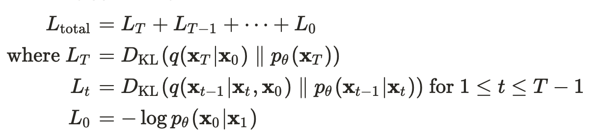
• NNL(negative log likelihood): 훈련은 NNL을 최적화하여 수행
  • $\mathbb{E}[-\text{log}p_\theta(\mathbf{x}0)] \le \mathbb{E}q[-\text{log}\frac{p\theta(\mathbf{x}{0:T})}{q(\mathbf{x}_{1:T}|\mathbf{x}0)}] \\ = \mathbb{E}q[-\text{log}p(\mathbf{x}T) - \Sigma{t\ge1}\text{log}\frac{p\theta(\mathbf{x}{t-1}|\mathbf{x}_t)}{q(\mathbf{x}t|\mathbf{x}{t-1})}] := L$

stochastic gradient descent으로 $L$의 random 항을 최적화함으로 효율적인 훈련이 가능하다. (Appendix A)

(모든 KL divergences는 Gaussian 분포들의 비교)

** KL divergences (from wiki)

: a measure of how one probability distribution P is different from a second, reference probability distribution Q.(=어떤 이상적인 분포에 대해, 그 분포를 근사하는 다른 분포를 사용해 샘플링을 한다면 발생할 수 있는 정보 엔트로피  차이를 계산한다.)

$D_{KL}(P||Q) = \Sigma P(x)log(\frac{P(x)}{Q(x)})$

** connections: Log likelihood, KL Divergence

The parameters that minimize the KL divergence are the same as the parameters that minimize the cross entropy and the negative log likelihood!

3. Diffusion models and denoising autoencoders

[detail은 논문 참고]

forward 프로세스의 분산 $\beta_t$와 reverse 프로세스의 model architecture, Gaussian distribution parameterization(mu)을 선택해야한다.

1. Forward process: $\beta_t$를 상수 취급(are fixed)하기 때문에 $L_T$상수취급하여 훈련에서 무시
2. Reverse process ($L_{1:T-1}$):
   • $\mu_\theta$를 평균 근사 훈련을 하여 $\tilde\mu_t$를 예측하거나 parameterization을 수정하여 $\epsilon$을 예측하도록 훈련.
   • $\mu_\theta(\mathbf{x}_t, t) = \tilde{\mu}_t(\mathbf{x}_t, \frac{1}{\sqrt{\hat\alpha_t}}\big(\mathbf{x}t - \sqrt{1-\bar\alpha_t}\epsilon\theta(\mathbf{x}_t))\big) = \frac{1}{\sqrt\alpha_t}\big(\mathbf{x}t - \frac{\beta_t}{\sqrt{1-\bar\alpha_t}}\epsilon\theta(\mathbf{x}_t, t)\big)$
   • (${\bf x}_{0}$을 예측할 수 있지만 실험 초기에 샘플 품질이 더 나빠지는 것으로 나타남)
3. Data scaling ($L_0$):(샘플링이 끝나면 $\mu_\theta({\bf x}_1,1)$ 를 noise를 제거하고 표시한다.)
   • 0 ~ 255로 구성되어있는 이미지 데이터는 $[-1, 1]$에서 선형 확장된다. 이렇게 하면 reverse process가 standard normal 사전분포 $p(\mathbf{x}_T)$에서 시작하여 일관되게 확장된 입력에 작동한다.
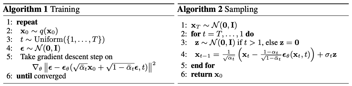
4. Simplified training objective
   • Algorithm 1, 단순화된 objective를 이용한 전체 training 프로세스
     • variational bound의 변형에 대해 학습하는 것이 sample 품질(구현 더 간단)에 더 유리하다는 것을 발견함:
     • $L_{simple}(\theta) := \mathbb{E}_{t,{\bf x}0, \epsilon} [ ||\epsilon - \epsilon_\theta(\sqrt{\bar\alpha}{\bf x}_0 + \sqrt{1-\bar\alpha_t}\epsilon,t)||^2]$
   • Algorithm 2, 전체 샘플링 프로세스는 데이터 밀도의 학습된 gradient로 $\theta$를 사용하는 Langevin dynamics 과 유사하다. ($\epsilon_{\theta}$is a function approximator intended to predict $\epsilon$ from ${\bf x}_t$)

4. Experiments

[Details are in Appendix B.]

Our neural network architecture follows the backbone of PixelCNN++ [52], which is a U-Net [48] based on a Wide ResNet [72].

We replaced weight normalization [49] with group normalization [66] to make the implementation simpler.

Our 32 × 32 models use four feature map resolutions (32 × 32 to 4 × 4), and our 256 × 256 models use six.

All models have two convolutional residual blocks per resolution level and self-attention blocks at the 16 × 16 resolution between the convolutional blocks [6].

Diffusion time $t$ is specified by adding the Transformer sinusoidal position embedding [60] into each residual block.

정리하다 발견한 디테일한 노션정리: https://sang-yun-lee.notion.site/Denoising-Diffusion-Probabilistic-Models

읽어보면 좋은 논문)

Dall-e 2 : https://arxiv.org/pdf/2102.12092.pdf  (OpenAI)

Imagen : https://gweb-research-imagen.appspot.com/paper.pdf (Google Research, Brain)