매일매일 딥러닝

• ref
  • Article: https://arxiv.org/pdf/2106.04939.pdf (2021)
  • code 없음

Keywords: Multimodal representation learning, Keyword extraction, Transformer, Graph embedding, (Key-phrase extraction)

Models: Bert(Transformer) & ExEm(Graph Embedding) → Random Forest Metric: F1-score

의견

논리적으로 좋은 아이디어인듯!

• text embedding, node(structure) embedding 두 모델의 앙상블
• random forest로 BIO tagging classification (with f-1 score)

단,

• code가 없어 당장 써보기 어려움 (ExEm 대신 node2vec 사용해봐도 될듯)
• 다만, 우선 구조적으로 graphical dataset을 만들어?찾아?야하지 않나? and 우리의 데이터셋은 structure(relationship)를 배울 필요성이 있나? 고민해보기

Graphs Neural Networks in NLP

“Its size is ideal and the weight is acceptable.”
 Attention-based models often identify acceptable as a descriptor of the aspect size, which is in fact not the case.

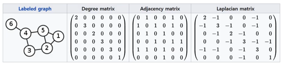
→ sentences as dependency graphs로?→ 생성을 어떻게 하지? → en의 경우 parser 있음

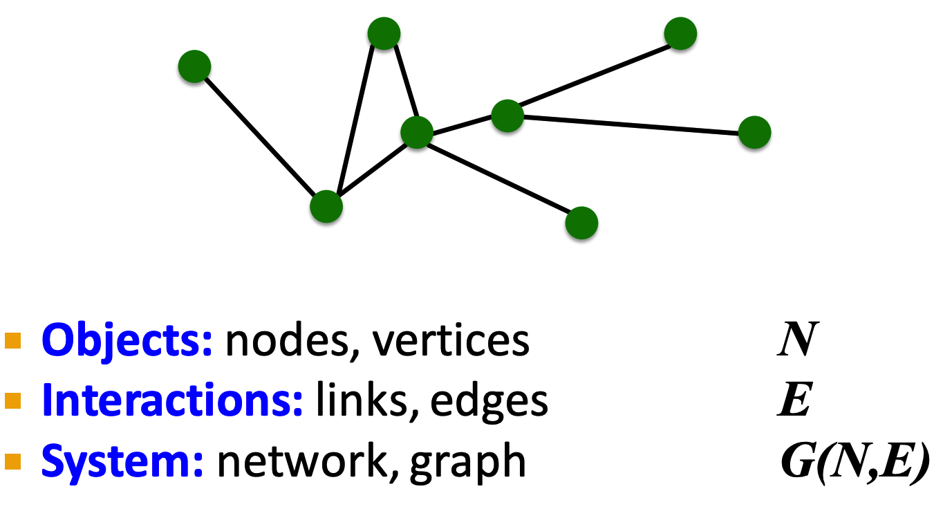
* graphs neural net의 장점: un( or semi)supervised learning, unkown relation(edge) embedding 가능

⇒ 사용할만한 keyphrase idea: BERT-RandomForest(BIO tagging)

Abstract

1. Background

Keywords are terms that describe the most relevant information in a document.

However, previous keyword extraction approaches have utilized the text and graph features, there is the lack of models that can properly learn and combine these features in a best way.

2. Methods

In Phraseformer, each keyword candidate is presented by a vector which is the concatenation of the text and structure learning representations.

Phraseformer takes the advantages of recent researches such as BERT(Sentence Embedding) and ExEm(Graph Embedding) to preserve both representations.

Also, the Phraseformer treats the key-phrase extraction task as a sequence labeling problem solved using classification task.

3. Results

F1-score, three datasets(Inspec dataset, ..) used

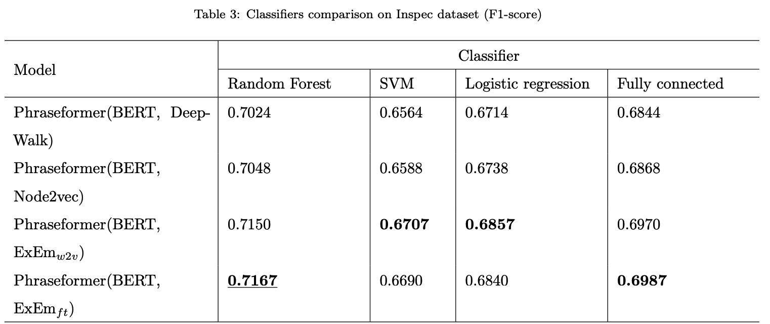
Additionally, the Random Forest classifier gain the highest F1-score among all classifiers.

4. Conclusions

Due to the fact that the combination of BERT and ExEm is more meaningful and can better represent the semantic of words.

Experimental Evaluation & Results

1. Dataset

Inspec includes abstracts of papers from Computer Science collected between the years 1998 and 2002. SE-2010 contains of full scientific articles that are obtained from the ACM Digital Library. In our experiment, we used the abstract of papers. SE-2017 consists of paragraphs selected from 500 ScienceDirect journal papers from Computer Science, Material Sciences and Physics domains.

*Gold keys: the ground-truth keywords

2. Metrics

$\text{F1-score} = 2 \times \frac{\frac{Y\cap Y'}{Y'}\times \frac{Y\cap Y'}{Y}}{\frac{Y\cap Y'}{Y'} + \frac{Y\cap Y'}{Y}} = 2\times \frac{\text{precision}\times\text{recall}}{\text{precision}+\text{recall}}$

$\text{precision} = \frac{\text{number of correctly matched}}{\text{total number of extracted}} = \frac{TP}{TP+FP}$

$\text{recall} = \frac{\text{number of correctly matched}}{\text{total number of assigned}} = \frac{TP}{TP+FN}$

3. Baseline models

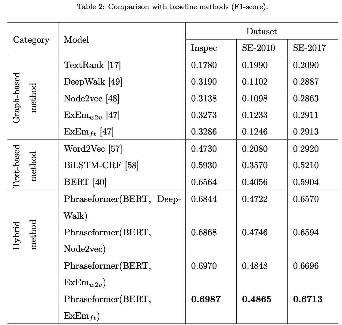
Node2vec [48] is modified version of DeepWalk that uses a biased random walks to convert nodes into vectors.

• Article: https://arxiv.org/abs/1607.00653
• code: https://github.com/aditya-grover/node2vec

1. We propose node2vec, an efficient scalable algorithm for feature learning in networks that efficiently optimizes a novel network-aware, neighborhood preserving objective using SGD.
2. We extend node2vec and other feature learning methods based on neighborhood preserving objectives, from nodes to pairs of nodes for edge-based prediction tasks.

ExEm [47] is a random walk based approach that uses dominating set theory to generate random walks.

• Article: https://arxiv.org/abs/2001.08503
• official code: https://github.com/AzarKh/ExEm…?

• A novel graph embedding using dominating-set theory and deep learning is proposed.
• $ExEm_{ft}$ : It is a version of ExEm that engages fastText method to learn the node representation.
• $ExEm_{w2v}$: This one is another form of ExEm that allows to create node representations by using Word2vec approach.

BERT [40] is a textual approach that uses the transformer structure to obtain the document representation.

• Article: https://arxiv.org/abs/1810.04805
• official code: https://github.com/google-research/bert

4. Classifier (BIO tagging)

In this part of our experiment we aim to investigate which classifier is best suited for sequence labelling and classification tasks to find key-phrases.

• paper) https://arxiv.org/pdf/2006.11239.pdf (UC Berkeley)
• code) https://github.com/hojonathanho/diffusion
• original diffusion model paper) https://arxiv.org/pdf/1503.03585.pdf

•  요약
  1. forward diffusion process $q(\mathbf{x}t|\mathbf{x}{t-1})$: noise를 점점 증가 시켜 가면서 학습 데이터를 특정한(Gaussian) noise distribution으로 변환
  2. reverse generative process $p_\theta(\mathbf{x}_{t-1}|\mathbf{x}_t)$: noise distribution으로부터 학습 데이터를 복원(=denoising)하는 것을 학습단 위과정을 Markov Chain으로 표현.
• 왜 잘될까?
  • 기존의 AutoEncoder와 같은 모델의 경우 Encoder 부분에서 어느 정도로 data가 encoding이 될지 알 수 없고 조절할 수 없었지만 Diffusion 모델의 경우 각 time step 마다 약간의 noise가 추가되고 reverse할 때 그 지정된 만큼(?), 종류(?)의 noise를 복원해내면 되기 때문이지 않을까..(마치 작은 tasks로 쪼개서 문제를 해결해나가듯)

1. Introduction

diffusion probabilistic model은 샘플에 매칭되는 데이터를 생성하기위해 variational inference를 사용하여 훈련된 parameterized Markov chain이다.

** Variational Inference 참고

(기계학습, Machine Learning) Week 1 Variational Inference | Lecture 1

** Markov chain: 마르코프 성질을 가진 이산 확률과정을 뜻합니다. (from wiki)

마르코프 성질은 과거와 현재 상태가 주어졌을 때의 미래 상태의 조건부 확률 분포가 과거 상태와는 독립적으로 현재 상태에 의해서만 결정된다는 것을 뜻한다.

이 Transition은 signal이 파괴될때까지(?= $x_0$까지) 샘플링의 반대반향으로 데이터에 노이즈를 점진적으로 추가하는 Markov chain의 diffusion process를 reverse하도록 학습된다.

diffusion이 적은 양의 Gaussian noise로 구성된 경우 샘플링 프로세스의 전환도 조건부 Gaussian으로 설정하면 충분하기때문에 간단한 neural network parameterization이 가능하다.

또한 diffusion model의 특정 parameterization은 훈련 중 multiple noise level에서 denoising score matching하는 것과 샘플링 중 Langevin dynamics 문제를 푸는 것과 동등하다는 것을 발견했다.

** Langevin dynamics (https://yang-song.github.io/blog/2021/score/)

Langevin dynamics provides an MCMC procedure to sample from a distribution $p(x)$ using only its score function $\nabla_\mathbf{x}\text{log} p(\mathbf{x})$.

$s_\theta \approx \nabla_\mathbf{x}\text{log} p(\mathbf{x})$

[Using Langevin dynamics to sample from a mixture of two Gaussians.]

이 논문에서는 diffusion model의 샘플링 프로세스가 autoregressive 모델로 일반화가 가능하다는 것과 autoregressive의 decoding과 유사한 일종의 점진적 decoding이라는 것을 보여준다.

** autoregressive decoder: 과거의 자기 자신을 사용하여 현재의 자신을 예측하는 모델이다. (from wiki)

$X_t = c+\Sigma_{i=1}^p \varphi_iX_{t-1} + \varepsilon_t$

2. Background

Forward process(diffusion process: from data to noise)

• diffusion model이 다른 유형의 latent 모델과 구별되는 것은 대략적인 사후 확률$q(\mathbf{x}\_{1:T}|\mathbf{x}_0)$이 데이터에 variance shedule $\beta_1, \dots, \beta_T$ 에 따라 Gaussian noise를 점진적으로 추가하는 Markov Chain에 고정된다는 것이다.
  • $q({\bf x}_{1:T}|{\bf x}_0) := \Pi_{t=1}^T q({\bf x}_t|{\bf x}_{t-1}), \\ q({\bf x}_t|{\bf x}_{t-1}) := \mathcal{N}({\bf x}_t; \sqrt{1-\beta_t}{\bf x}_{t-1}, \beta_t \bf{I})$
• forward process에서는 cosed form timestep $t$에서 $\mathbf{x}_t$를 샘플링하는 것을 허용한다. (한번에 0에서 t번째 샘플을 얻는 방법)
  • $\alpha_t := 1-\beta_t, \bar\alpha_t := \Pi_{s=1}^t \alpha_s$
  • $q(\mathbf{x}_t|\mathbf{x}_0) = \mathcal{N}(\mathbf{x}_t;\sqrt{\bar\alpha_t}\mathbf{x}_0, (1-\bar\alpha_t)\mathbf{I})$

Reverse process(generative process: from noise to data)

• diffusion 모델은 $p_\theta(\mathbf{x}0):= \int p\theta(\mathbf{x}_{0:T})$형식의 latent variable 모델이다.
  • ($\mathbf{x}_1, \cdots, \mathbf{x}_T$는 $\mathbf{x}_0 \sim q(\mathbf{x}_0$)과 같은 차원의 latents를 갖는다.)
• $p_\theta(x_{0:T})$는 reverse process라고 하며 Markov chain으로 $p(\mathbf{x}_T)=\mathcal{N}(x_T;0, \mathbf{I})$에서 시작하는 trained Gaussian Transition 으로 정의된다.

Objective

• NNL(negative log likelihood): 훈련은 NNL을 최적화하여 수행
  • $\mathbb{E}[-\text{log}p_\theta(\mathbf{x}0)] \le \mathbb{E}q[-\text{log}\frac{p\theta(\mathbf{x}{0:T})}{q(\mathbf{x}_{1:T}|\mathbf{x}0)}] \\ = \mathbb{E}q[-\text{log}p(\mathbf{x}T) - \Sigma{t\ge1}\text{log}\frac{p\theta(\mathbf{x}{t-1}|\mathbf{x}_t)}{q(\mathbf{x}t|\mathbf{x}{t-1})}] := L$

stochastic gradient descent으로 $L$의 random 항을 최적화함으로 효율적인 훈련이 가능하다. (Appendix A)

(모든 KL divergences는 Gaussian 분포들의 비교)

** KL divergences (from wiki)

: a measure of how one probability distribution P is different from a second, reference probability distribution Q.(=어떤 이상적인 분포에 대해, 그 분포를 근사하는 다른 분포를 사용해 샘플링을 한다면 발생할 수 있는 정보 엔트로피  차이를 계산한다.)

$D_{KL}(P||Q) = \Sigma P(x)log(\frac{P(x)}{Q(x)})$

** connections: Log likelihood, KL Divergence

The parameters that minimize the KL divergence are the same as the parameters that minimize the cross entropy and the negative log likelihood!

3. Diffusion models and denoising autoencoders

[detail은 논문 참고]

forward 프로세스의 분산 $\beta_t$와 reverse 프로세스의 model architecture, Gaussian distribution parameterization(mu)을 선택해야한다.

1. Forward process: $\beta_t$를 상수 취급(are fixed)하기 때문에 $L_T$상수취급하여 훈련에서 무시
2. Reverse process ($L_{1:T-1}$):
   • $\mu_\theta$를 평균 근사 훈련을 하여 $\tilde\mu_t$를 예측하거나 parameterization을 수정하여 $\epsilon$을 예측하도록 훈련.
   • $\mu_\theta(\mathbf{x}_t, t) = \tilde{\mu}_t(\mathbf{x}_t, \frac{1}{\sqrt{\hat\alpha_t}}\big(\mathbf{x}t - \sqrt{1-\bar\alpha_t}\epsilon\theta(\mathbf{x}_t))\big) = \frac{1}{\sqrt\alpha_t}\big(\mathbf{x}t - \frac{\beta_t}{\sqrt{1-\bar\alpha_t}}\epsilon\theta(\mathbf{x}_t, t)\big)$
   • (${\bf x}_{0}$을 예측할 수 있지만 실험 초기에 샘플 품질이 더 나빠지는 것으로 나타남)
3. Data scaling ($L_0$):(샘플링이 끝나면 $\mu_\theta({\bf x}_1,1)$ 를 noise를 제거하고 표시한다.)
   • 0 ~ 255로 구성되어있는 이미지 데이터는 $[-1, 1]$에서 선형 확장된다. 이렇게 하면 reverse process가 standard normal 사전분포 $p(\mathbf{x}_T)$에서 시작하여 일관되게 확장된 입력에 작동한다.
4. Simplified training objective
   • Algorithm 1, 단순화된 objective를 이용한 전체 training 프로세스
     • variational bound의 변형에 대해 학습하는 것이 sample 품질(구현 더 간단)에 더 유리하다는 것을 발견함:
     • $L_{simple}(\theta) := \mathbb{E}_{t,{\bf x}0, \epsilon} [ ||\epsilon - \epsilon_\theta(\sqrt{\bar\alpha}{\bf x}_0 + \sqrt{1-\bar\alpha_t}\epsilon,t)||^2]$
   • Algorithm 2, 전체 샘플링 프로세스는 데이터 밀도의 학습된 gradient로 $\theta$를 사용하는 Langevin dynamics 과 유사하다. ($\epsilon_{\theta}$is a function approximator intended to predict $\epsilon$ from ${\bf x}_t$)

4. Experiments

[Details are in Appendix B.]

Our neural network architecture follows the backbone of PixelCNN++ [52], which is a U-Net [48] based on a Wide ResNet [72].

We replaced weight normalization [49] with group normalization [66] to make the implementation simpler.

Our 32 × 32 models use four feature map resolutions (32 × 32 to 4 × 4), and our 256 × 256 models use six.

All models have two convolutional residual blocks per resolution level and self-attention blocks at the 16 × 16 resolution between the convolutional blocks [6].

Diffusion time $t$ is specified by adding the Transformer sinusoidal position embedding [60] into each residual block.

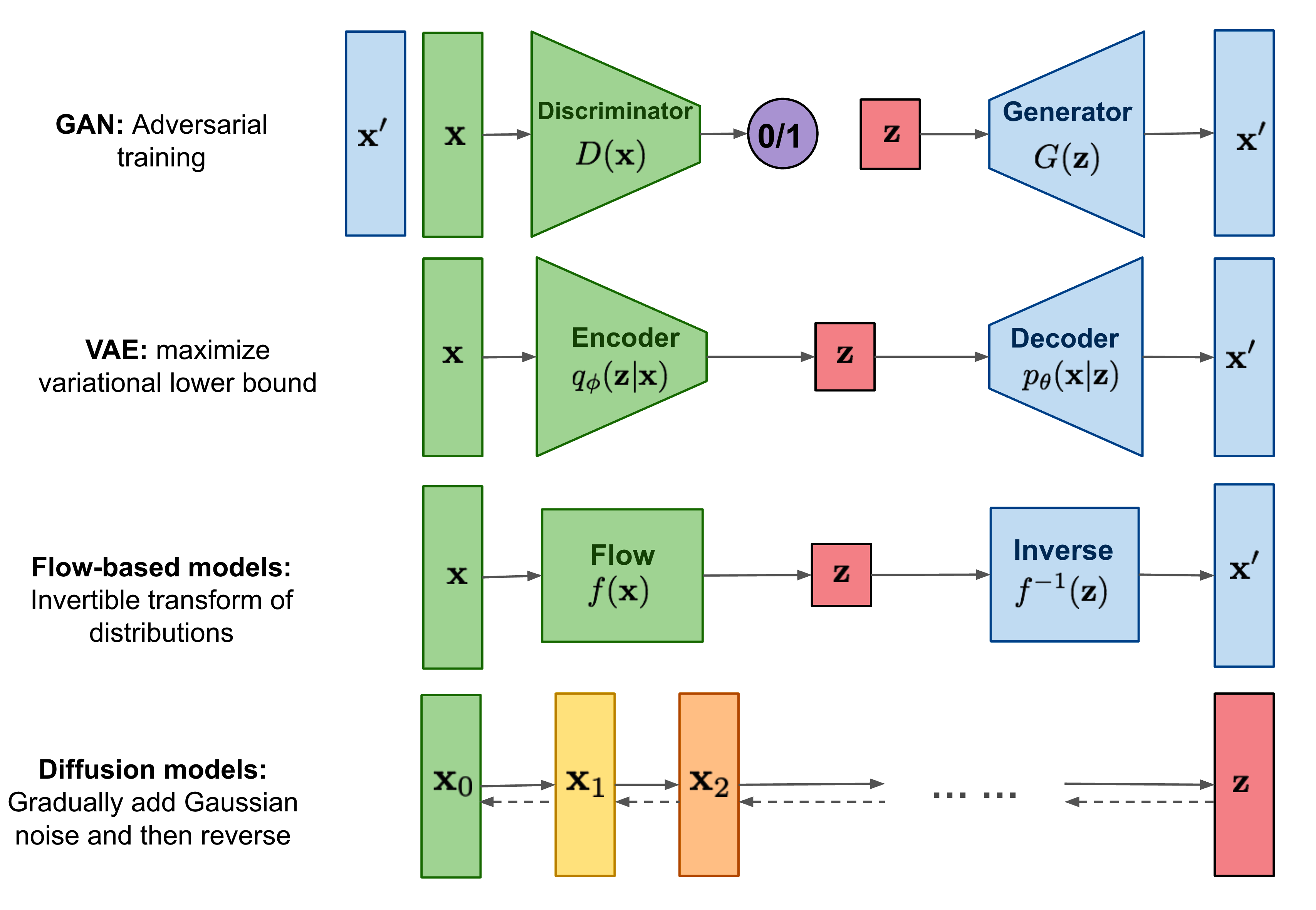
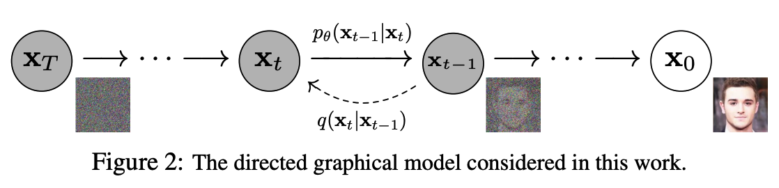
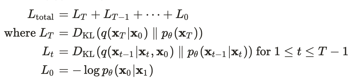
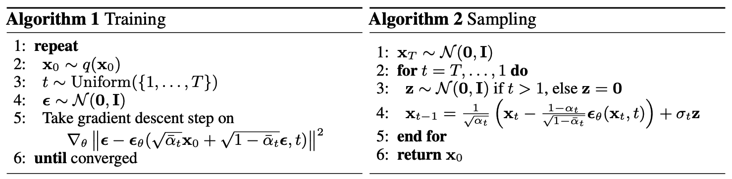
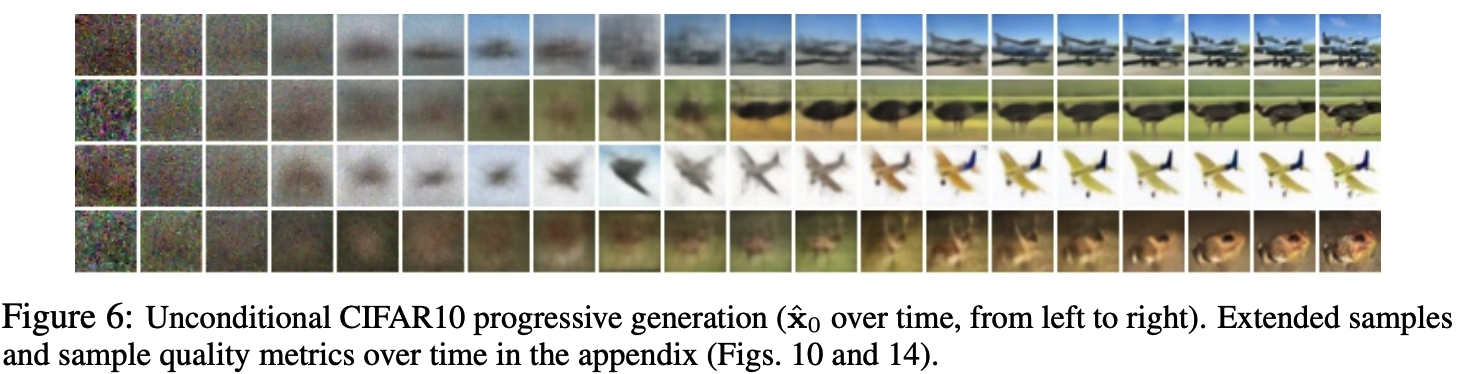
정리하다 발견한 디테일한 노션정리: https://sang-yun-lee.notion.site/Denoising-Diffusion-Probabilistic-Models

읽어보면 좋은 논문)

Dall-e 2 : https://arxiv.org/pdf/2102.12092.pdf  (OpenAI)

Imagen : https://gweb-research-imagen.appspot.com/paper.pdf (Google Research, Brain)

(이 포스팅에서는 논문 전체를 다루지 않고 Graph-based SSL의 기초적인 부분(Chapter4.A까지)만 다룹니다.)

• paper
  https://arxiv.org/pdf/2102.13303.pdf
• reference
  https://www.youtube.com/watch?v=HM5z8bH29Ag&list=PLetSlH8YjIfWMdw9AuLR5ybkVvGcoG2EW&index=34
  https://junhyungbyun.github.io/Graph-based-Semi-Supervised-Learning/

Abstract

Semi-supervised learning (SSL)은 labeld data와 unlabeled data 모두를 통합하는 기능이 있기 때문에 상당한 가치가 있다. Graph-based semi-supervised learning (GSSL)은 다양한 도메인에서 장점이 있다는 것이 입증되었다. 논문의 주요한 기여는 graph regularization과 graph embedding methods를 포함한 GSSL의 새로운 일반화 분류법에 있다.

1. Introduction

Graph-based SSL (GSSL)은 graph 구조상 중요한 manifold를 압축하여 반영하여 자연스럽게 사용될 수 있기때문에 특히 유망하다. graph는 구조적으로 nodes는 모든 samples를 표현할 수 있고 weighted edges는 nodes의 쌍 사이의 유사성을 반영한다.

[GSSL의 주요 과정]

Step 1. Graph construction.

A similarity graph는 labeled, unlabeled samples를 포함한 데이터로 구성되어있다.

original samples사이의 관계를 잘 표현하는 것이 중요한 과제이다.

Step 2. Label inference.

이전 step에서 만들어진 graph 구조 정보를 통합하여 labeled samples로 부터 unlabeled samples로 label 정보를 전파하는 것을 수행한다.

(this paper) Label inference methods are then categorized into two main groups: graph regularization methods and graph embedding methods. [논문참고]

2. Background and Definition

A Comprehensive Survey on Graph Neural Networks

[논문참고]

3. Graph construction

• Goal: $G = (V,E,W)$, V: nodes set, E : edges, W: associate weights(=인접행렬)
• Assumption
  1. undirected graph임 → W: symmetric
  2. edge weights는 non-negative → $W_{ij} \ge 0, \forall i \ne j$
  3. no self-loop
• Edges: similarity weights computed from featureshttps://junhyungbyun.github.io/Graph-based-Semi-Supervised-Learning/
• : x3는 similarity weights(=edge)가 강한 x1과 같은 label을 가질 가능성이 높다

A. Unsupervised methods

기존의 보편적인 전략, graph 구성시 label 정보 무시

• k-nearest-neighbor graph→ 밀도는 고려하지 않음
• $W_{ij} = \begin{cases} sim({\bf x}_i, {\bf x}_j) & i\in \mathcal{N}(j) \\ 0 & otherwise \end{cases}$
• b-Matching:
  • (a) graph sparsification (edge selection)$P\in {0,1}^{n\times n}$, 1: egde 존재$\Delta \in \mathcal{R}_{+}^{n\times n}$ : symmetric distance matirx
  • $\Sigma_j P_{ij} = b, P_{ii}=0, P_{ij}=P_{ji}, \forall 1 \le i, i \le n$
  • $min_{P\in{0,1}^{n\times n}} \Sigma_{i,j} P_{ij} \Delta_{ij}$
  • (b) edge re-weighting ($W$구하기)
    • Binary kernel, Gaussian kernel(=RBF Kernel), Locally linear reconstruction
    • → similarity graph construction시 제한을 줌 ⇒ label inference시 더 균형잡힌 전파 가능

B. Supervised methods

lable 정보를 prior knowledge로서 graph 생성시 사용할 수 있다. ⇒ supervised information를 추가하면 inference 과정을 촉진할 수 있다.

C. ETC(논문에는 언급되지 않음)

fully connected graph: weight decays with distance  $w_{ij} = exp(\frac{-||x_i - x_j||^2}{\sigma^2})$

$\epsilon$-radius graph (k-nn과 유사하지만 개수를 제한하지 않음, 단 주변 노드가 없을 수 있음)

4. Graph regularization

• general regularization framework
• $\mathcal{L}(f) = \Sigma_{(x_i,y_i)\in\mathcal{D}}\underbrace{\mathcal{L}_s(f(x_i),y_i)}{supervised\ loss} + \mu \ \Sigma_{x\in\mathcal{D}l+\mathcal{D}_u}\underbrace{\mathcal{L}_r(f(x_i))}{regularization\ loss}$

A. label propagation

주어진 label은 fix해야함. labeled nodes의 정보가 edges를 통해 unlabeled nodes로 label을 예측할 때 가이드하는 역할을 한다.

[basic label propagation 알고리즘]

Step 1. All nodes propagate labels for one step $Y\leftarrow TY$

Step 2. Row-normalize Y to maintain the class probability interpretation.

Step 3. Clamp the labeled data. Repeat from step 2 until Y converges.

1) Gaussian random fields

이차 손실함수의 경우 infinity weight를 가짐 → closed-form으로 만드는 harmonic function을 사용

** Harmonic function: unlabeled data의 경우 descrete labels({0,1})를 continuous values로 표현할 수 있다.

$E(f) = \mathcal{L}_r = \frac{1}{2}\Sigma_{i,j} W_{ij}(f(x_i)-f(x_j))^2$

$f(x_i) = f_l(x_i) \equiv y_i$, $f$를 최소화

• unlabeled nodes는 제약조건 $Lf = 0$을 만족함
• unlabeled node는 neighbor nodes의 평균
• $f(x_j) = \frac{1}{d_j}\Sigma_{i\sim j} W_{ij}f(x_i)$, $j = l+1, \dots, l+u$
• 반복적인 방식으로 해석: $f^{(t+1)} \leftarrow P\cdot f^{(t)}$, $P = D^{-1}W$

$L$: Laplacian matrix

• Diagonal degree matrix$D: D_{ii} = \Sigma_{j=1}^nW_{ij}$ ** degree: node에 연결된 edges 개수
• Graph Laplacian matrix
  • $\Delta = D-W$

→ 가중치 행렬을 4 blocks로 분할하면 추론가능

$W = \begin{bmatrix} W_{ll} & W_{lu} \ W_{ul} & W_{uu} \end{bmatrix}$

$f_u = (D_{uu}-W_{uu})^{-1}W_{ul}f_l = (I-P_{uu})^{-1}P_{ul}f_l$

→ 단점)

(a) label을 fix하고 진행하여 noise에 약함 (유연하지 않음)

(b) 새로운 test points에 대해서 직접적으로 적용할 수 없음 (Figure 2. Transductive)

2) Local and global consistency(LGC)

$\mathcal{L}(f) = \frac{1}{2}(\Sigma_{i,j} W_{ij}(\frac{1}{\sqrt{D_{ii}}}f(x_i)- \frac{1}{\sqrt{D_{jj}}}f(x_j))^2)+\mu\ \Sigma_{i=1}^{n_l}(f(x_i)-y_i)^2$

→ GRF와 다른점:

(a) labeled node가 seed label과 같지 않을 수 있음 (=유연함, noise가 있을 때 유리)

(b) $\frac{1}{\sqrt{D_{ii}}}$(degree)로 각 node의 label에 penalty를 줄 수 있음. 상위 nodes의 영향력을 regularization할 수 있고 불규칙한 graph에도 보장함

Components of Graph Network

A Comprehensive Survey on Graph Neural Networks

• paper: https://arxiv.org/pdf/1901.00596.pdf

image classification, natural language understanding 등 기존 tasks의 데이터는 Euclidean space에서 표현했다. 하지만 application 수가 증가하며 생성된 데이터는 non-Euclidean domains이고 이는 object 사이에 복잡한 관계를 갖는 graph로 표현된다.

1. Introduction

graphs는 불규칙적일 수 있다. 다양한 순서가 없는 node를 가질수도, node에 연결된 nieghbors의 숫자도 다를 수 있다. 따라서 graph domain에는 다르게 적용해야한다.

graph 데이터를 다루기위해 기존의 딥러닝 CNNs, RNNs, autoencoder 방법으로부터 새로운 일반화를 통한 응용한 연구가 진행되어왔다. 예를 들어 graph convolution은 2D convolution의 일반화가 될 수 있다. 2D convolution과 유사하지만 graph convolution은 node’s neighborhood 정보의 weight average를 가진다.

** manifolds: 국소적으로는 유클리드 공간과 닮았지만 대역적으로는 위상 공간이다.

2. BackGround & Definition

outlines the background of graph neural networks, lists commonly used notations, and defines graph-related concepts.

A. Background

A brief history of graph neural networks (GNNs)

이전 연구들은 recurrent graph neural networks의 카테고리였다. 고정된 point에 도달할때 까지 neighbor information을 전파하는 방법으로 target node’s representation을 학습한다. 하지만 이 프로세스는 컴퓨팅 비용이 비싸며 이 문제를 극복하기 위한 노력이 증가해왔다.

2009년에는 RNN(message passing)의 아이디어를 상속하면서 구조적으로 non-recursive layer를 합성하여 graph mutual dependency를 해결하는 RecGNNs(Micheli et al.) 방법이 제안되었다.

CV 도메인에서 CNN의 성공으로 graph를 데이터를 병렬적 개발하기 위한 convolution이 재정의되었다. ConvGCNNs(Bruna et al.(2013)) 은 spectral-based 접근법과 spatial-based 접근법으로 주요하게 나눠진다.

Graph neural networks vs. network embedding

network embedding의 목적은 low-dimensional vector로 representation을 생성하고 network topology structure와 node content information을 모두 보존하여 classification, clustering, recommendation등을 쉽게 수행할수 있도록 하는 것이다. matrix factorization, random walks 방법(non-deep learning method)을 사용한다. (예시, support vector machines for classification)

GNNs은 딥러닝 모델이며 end-to-end graph와 연관된 task를 해결하는 것이 목적이다. GNNs는 다양한 task를 위한 neural network model의 그룹이며 다양한 network embedding을 포함하고 있다.

Graph neural networks vs. graph kernel methods

GNNs과 유사하게 graph kernels는 mapping function을 이용하여 graphs or nodes를 vector space로 임베딩할 수 있다. mapping function이 learnable하기보다는 deterministic하다는 점이 다르다.

B. Definition

Definition 1 (Graph):

$G=(V,E)$, $V$: nodes, $E$: set of edges

$v_i \in V, e_{ij} = (v_i, v_j) \in E$

neighborhood of a node $N(v) = {u\in V|(v,u) \in E}$

adjacency matrix $A$ is $n \times n$ matrix 

** 인접 행렬: edges의 관계를 표현

$\begin{cases} A_{ij} = 1 ,\ if\ e_{ij} \in E \ A_{ij} = 0,\ if\ e_{ij} \notin E \end{cases}$

node attributes matrix $X \in R^{n\times d}$

node feature attribute $x_v \in R^d$

edge attribute $X^e \in R^{m\times c}$

edge feature attribute $x_{v,u}^e \in R^c$

Definition 2 (Directed Graph):

directed(방향이 있는) graph는 node로부터 다른 node로 향하는 edges가 있는 것이다. adjacecy matrix가 대칭적인 경우에만 undirected graph이다.

Definition 3 (Spatial-Temporal Graph):

$G^{(t)} = (V,E,X^{(t)}), X^{(t)} \in R^{n\times d}$ : node attributes matrix도 고려!

spatial-temporal graph는 node attributes가 시간에 따라 dynamic하게 변화하는 attributed graph이다.

3. Categorization and Frameworks

clarifies the categorization of graph neural networks

A. Taxonomy of Graph Neural Netowrks (GNNs)

Recurrent graph neural networks (RecGNNs): GNN의 개척자라고 볼 수 있다.

RecGNN의 목적은 recurrent neural architectures로 node representation을 학습하는 것이다. graph의 node은 stable equilibrium(=변화하지 않는 안정된 상태)에 도달할 때까지 neighbor와 정보를 교환한다고 가정한다.

Convolutional graph neural networks (ConvGNNs): grid data로 부터 graph data로 convolution 연산을 일반화한다.

주된 아이디어는 feature $x_v$ 와 neighbors’ features $x_u$(where $u \in N(v)$)를 조합하여 node $v$’s features $x_u$를 생성하는 것이다. RecGNNs와 달리 ConvGNNs는 high-level node representation을 추출하기 위해 multiple graph convolutional layers를 쌓는다.

Figure 2a shows a ConvGNN for node classification.

Figure 2b demonstrates a ConvGNN for graph classification.

Graph autoencoders (GAEs): unsupervised learning framework이다.

node/graph를 latent vector space로 인코딩하고 encoded information으로부터 graph data를 재구성한다. network embedding과 graph generative distribution을 학습하는데 유용한다.

Figure 2c presents a GAE for network embedding.

Spatial-temporal graph neural networks (STGNNs): hidden patterns를 학습하는 것이 목적이다.

핵심 아이디어는 spatial dependency와 temporal dependency를 한번에 고려하는 것이다.

Figure 2d illustrates a STGNN for spatial-temporal graph forecasting.

B. Frameworks

mechanisms

• Node-level outputs relate to node regression and node classification tasks. With a multi-perceptron or a softmax layer as the output layer, GNNs are able to perform node-level tasks in an end-to-end manner.
• Edge-level outputs relate to the edge classification and link prediction tasks. two nodes’ hidden representations로 the label/connection strength of an edge 예측할 수 있다.
• Graph-level outputs relate to the graph classification task. graph level에서 compact representation를 얻을 수 있다.

Training Frameworks

Many GNNs (e.g., ConvGNNs) can be trained in a (semi-) supervised or purely unsupervised way within an end-to-end learning framework, depending on the learning tasks and label information available at hand.

• Semi-supervised learning for node-level classification
• Supervised learning for graph-level classification
• Unsupervised learning for graph embedding