매일매일 딥러닝

• 논문
  
  • https://arxiv.org/pdf/2004.00049.pdf
• code
  • https://genforce.github.io/idinvert/

** 아래의 내용과 이미지는 위의 논문을 기반으로 작성하였습니다.

** 수정할 부분이나 의견이 있다면 댓글로 달아주세요~

[참고] 미리보기

• Source: https://www.youtube.com/watch?v=TVSJO9uNq7g

GAN Inversion : GAN을 거꾸로 하는 것

: real image를 latent space의 적절한 latent code로 Inversion하는 task

→ latent space를 배운다. (explainable)

⇒ latent space 상의 각각의 latent code로 부터 realistic한 image를 얻을 수 있다.

StyleGAN: 각 layer 마다 hierarchical latent code를 부여하여 generation

: 위의 구조는 realistic한 output을 얻을 수 있을뿐만 아니라 각 layer별로 latent vector의 의미가 다르게 훈련됨 → output 이미지를 조절할 수 있다.

Abstract

기존 GAN의 경우 real image를 editing하기위한 semantics를 배우기 어려웠다.

현존하는 inversion methods는 pixel 기준으로 target image를 reconstucting(재구성)하기 때문에 original latent space에 semantic한 inverted code를 배치시키는데 실패했다.

논문에서는 이러한 문제를 해결하기 위해 in-domain GAN inversion방식을 제안한다. input image를 reconstuct할 뿐아니라 image editing을 위한 semantically meaningful latent code로 invert할 수 있다.

→ in domain ( latent space 안에서) GAN inversion을 제시, real image에 semantic한 editing할 수 있다.

1 Introduction

• in domain 예: like face, tower, bedroom
• semantic 예 : eyeglasses, smile (→ face에서 자연스럽게?)

GAN은 image를 생성하는 generator와 실제 이미지와 가짜 이미지를 판별하는 discriminator로 구성되어있다.

최근 연구에서 GAN이 latnet space에서 풍부한 semantics를 encoding하는 방법으로 학습하고 latent code를 변경하면 output image에서 해당하는 attributes를 조작(manipulation)할 수 있다는 것을 보여줬다.

하지만, real image를 입력으로 사용하여 latent code를 추론하는 기능이 없기 때문에 이러한 manipulation을 적용하기에는 여전히 어렵다.

GAN Inversion으로 image sapce를 latent space로 mapping하여 generation process로 되돌리려는 시도가 많이 있지만, 기존 방법은 주로 input image의 pixel을 기준으로 reconstruct하는 것에 중점을 두었다.

하지만 이 논문에서는 GAN Inversion 작업에서 pixel 수준 뿐 아니라 latent space에 encoding된 semantic knoledge와 align되어야한다고 주장한다. 이런 semantically meaningful codes는 GAN이 학습한 domain에 종속되기 때문에 in-domian code라고 부른다.

2 In-Domain GAN Inversion

GAN Invert할 때 input image의 pixel값을 복구하는 것 외에도 inverted code가 semantically 의미있는지 여부도 고려한다.

여기서 semantics는 GAN이 관찰된 data로부터 학습한 emergent knoledge를 의미한다.

방법: as shown in Fig.2.

1. novel domain-guided encoder를 훈련하여 encoder에서 생성된 모든 code가 domain내에 있도록 image space를 latent space에 매핑한다.
2. inverted code의 semantic property에 영향을 주지않고 pixel 값을 더 잘 reconstruct하기위해 instance-level domain-regularized optimization한다.

Problem Statement.

GAN model은 generator G(·) : Z → X 와 discriminator D(·) 로 구성되어있다. GAN Inversion은 주어진 실제 이미지 x real을 복구하기 위해 최상의 잠복 코드 z inv를 찾는 reverse mapping of G(·)을 학습한다.

Choice of Latent Space.

일반적으로 GAN은 미리 정의된 distribution space (such as normal distibution) Z에서 latent code z를 샘플링한다.

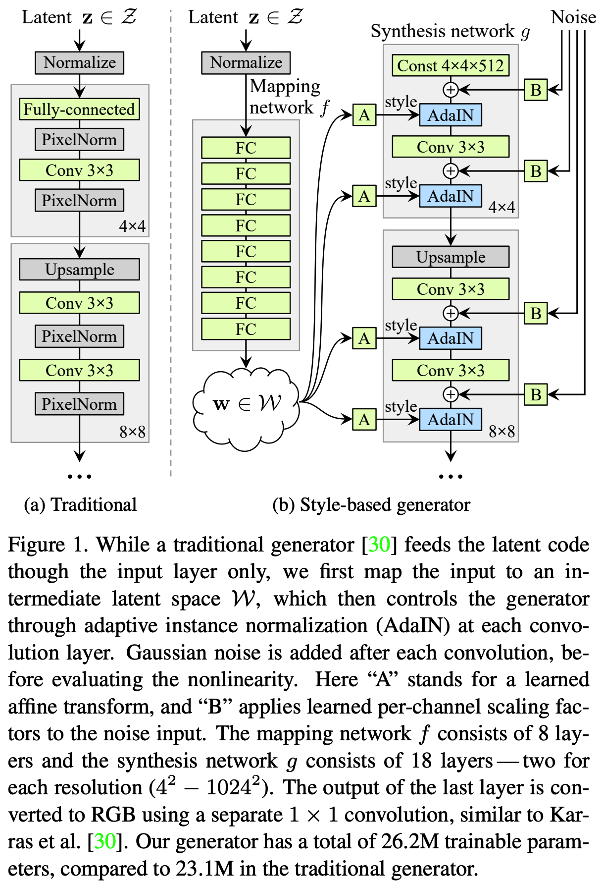
최근 StyleGAN 모델은 Multi-Layer Perceptron (MLP)를 이용하여 initial latent space Z를 두번째 latent space W에 매핑한다음 w ∈ W를 Generator에 사용하는 (additional mapping) 방법을 제안했다. → GAN inversion task에서 많이 사용됨

3가지 이유로 이 논문에서도 inversion space로 W space를 선택한다.

(i) We focus on the semantic (i.e., in-domain) property of the inverted codes, making W space more appropriate for analysis.

(ii) Inverting to W space achieves better performance than Z space [35].

( but our approach can be performed on the Z space as well. For simplicity, we use z to denote the latent code in the following sections. )

(iii) It is easy to introduce the W space to any GAN model by simply learning an extra MLP ahead of the generator.

2.1 Domain-Guided Encoder

Fig.2(a)의 위에 있는 (conventional encoder)를 보면, latent codes $z^{sam}$는 랜덤하게 샘플링되어 Generator에 들어가고 연관된 synthesis $x^{syn}$ 이미지를 얻는다.

그리고 Encoder는 $x^{syn}$ 를 input으로 $z^{sam}$ supervisions으로 하고 eq1으로 훈련된다.

$min_{\Theta_E}L_E = ||z^{sam} - E(G(z^{sam}))||_2$, (1)

where $||·||_2$ denotes the $l_2$ distance and $\Theta_E$ represents the parameters of the encoder E(·).

→ it is not powerful enough to train an accurate encoder and cannot provide its domain knowledge

이러한 문제를 해결하기위해 저자는 domain-guided encoder(in the bottom row of Fig.2(a))를 제안한다.

→ 기존 gan 방법과 달리 latent space가 아닌 real image space에서 input image를 reconstruct 함 : G(E(xreal))

1. The output of the encoder is fed into the generator to reconstruct the input image such that the objective function comes from the image space instead of latent space.
2. Instead of being trained with synthesized images, the domain-guided encoder is trained with real images, making our encoder more applicable to real applications.
3. To make sure the reconstructed image is realistic enough, we employ the discriminator to compete with the encoder. (both two components of GAN are used).

이 방식으로 GAN 모델에서 최대한 많은 정보를 얻을 수 있다.

The training process can be formulated as LE, LD

$$min_{\Theta_E}L_E = ||x^{real}-G(E(x^{real}))||2 \\ + \lambda{vgg} ||F(x^{real}) - F(G(E(x^{real})))||2 \\ - \lambda{adv} \mathbb{E}{x^{real} \sim P{data}}[D(G(E(x^{real})))],$$ (2)

• loss1: per pixel loss
  • $||x^{real}-G(E(x^{real}))||_2$ : x와 (x >> Encoder >> generator >>) z를 비교하는 loss,
• loss2: perceptual loss
  • F(·) denotes the VGG feature extraction model.
    • perceptual loss: Perceptual loss란 [11]에서 처음으로 제안된 손실 함수로 입력과 GT를 미리 학습해 놓은 다른 딥러 닝 기반의 영상 분류 네트워크에 통과 시킨 후 얻 은 feature map 사이의 손실을 최소화 하는 방향 으로 필터 파라미터를 학습한다.
    • source: http://www.kibme.org/resources/journal/20200504094149078.pdf
  • $\lambda_{vgg} ||F(x^{real}) - F(G(E(x^{real})))||_2$ : vgg loss 사용
• loss3: discriminator loss
  • Pdata denotes the distribution of real data
  • $\lambda_{adv} \mathbb{E}{x^{real} \sim P{data}}[D(G(E(x^{real})))]$ : discriminator를 training용

$$min_{\Theta_D} L_D = \mathbb{E}{x^{real} \sim P{data}}[D(G(E(x^{real})))] \\ - \mathbb{E}{x^{real} \sim P{data}}[D(x^{real})] \\ + \frac{\gamma}{2} \mathbb{E}{x^{real} \sim P{data}} [|| \nabla_x D(x^{real})||_2^2],$$ (3)

• loss 1: discriminator loss
  • $\mathbb{E}{x^{real} \sim P{data}}[D(G(E(x^{real})))] - \mathbb{E}{x^{real} \sim P{data}}[D(x^{real})]$ : 가짜(생성된 이미지), real image discriminator loss
• loss 2: gradient regularization
  • $\frac{\gamma}{2} \mathbb{E}{x^{real} \sim P{data}} [|| \nabla_x D(x^{real})||_2^2]$ : 변화량에 penalty
  • γ is the hyper-parameter

2.2 Domain-Regularized Optimization

distribution level에서 mapping을 학습하는 GAN의 generation process와 달리, GAN inversion은 주어진 개별 image를 가장 잘 reconstruct하는 instance-level task와 비슷하다.

이러한 관점에서 볼때 encoder 만으로는 representation capability이 제한되어 완벽한 reverse mapping을 학습하기 어렵다. 따라서, 여전히 code를 pixel 값에서 개별 target image와 더 잘 fit하게 수정해야한다.

The top row of Fig.2(b)에서 latent code는 generator만을 기반으로 'freely' 최적화된다.

이것은 latent code를 제약이 없기때문에 an out-of-domain inversion이 발생할 가능성이 매우 높다.

The bottom of Fig.2(b)에서 보이는 것처럼, 2가지 개선사항으로 domain-regularized optimization을 설계한다.

1. We use the output of the domain-guided encoder as an ideal starting point which avoids the code from getting stuck at a local minimum and also significantly shortens the optimization process.
2. We include the domain-guided encoder as a regularizer to preserve the latent code within the semantic domain of the generator.

To summarize, the objective function for optimization is

$$z^{inv} = argmin_z (||x - G(z)||2 \\+ \lambda{vgg}||F(x) - F(G(x))||2 \\+ \lambda{dom}||z-E(G(z))||_2),$$ (4)

• x is the target image to invert
• λvgg : the perceptual loss
• λdom: encoder regularizer respectively
  
  • $\lambda_{dom}||z-E(G(z))||_2$
  • z와 (z >> Generator >> Encoder >>) z' 을 같도록 훈련 ⇒ semantic 의미를 잘 갖추도록 (z를 이미 잘 구해놓았다는 전제하고 z를 fine-tuning, 최적화)

3 Experiments

[논문 참고]

4 Discussion and Conclusion

in domain으로 훈련해서 out of distribution에서는 별로다.(in Fig.10) → semantic한 훈련이 되었다는 의미로 볼 수 있다.

결론적으로, in-domain inversion은 pixel level과 semantic level 모두에서 대상 이미지를 복구하는 데 가장 적합한 (latent) code를 찾는 것을 목표로 하며 real image editing을 상당히 용이하게 한다.

[논문] arxiv.org/pdf/1703.04247.pdf

** 아래의 내용은 위의 논문을 기반으로 재해석한 내용입니다.
** 오타 혹은 부족한 부분이 있다면 첨언 및 조언 환영합니다!

[참고] 미리보기

1. CTR(click-through rate): 정의

클릭률(CTR)은 광고를 본 사용자가 해당 광고를 클릭하는 빈도의 비율입니다. 클릭률(CTR)을 사용하면 키워드와 광고, 무료 제품 목록의 실적을 파악할 수 있습니다.

• CTR은 광고가 클릭된 횟수를 광고가 게재된 횟수로 나눈 값입니다(클릭수 ÷ 노출수 = CTR)

Source: https://support.google.com/google-ads/answer/2615875?hl=ko

2. Factorization Machine

FM은 매트릭스 요소화(Matrix factorization)를 통해 문제의 치수(dimension)를 줄이는 기능에서 이름을 얻습니다.

Factorization Machine은 분류 또는 회귀에 사용될 수 있으며 선형 회귀와 같은 기존의 알고리즘보다 대형 스파스(sparse) 데이터셋에서 훨씬 더 효율적입니다.

Source: https://www.megazone.com/techblog_180709_movie-recommender-with-factorization-machines/

Abstract

추천 시스템에서 CTR을 최대화하는 것은 매우 중요하다.

하지만 기존의 방법은 lower- 혹은 high order 둘 중 하나에만 적용할 수 있었다.

따라서 이 논문에서는 lower-와 high order 의 interaction을 고려하며 feature engineering이 필요없는 end-to-end 학습 모델인 DeepFM을 제안한다.

• [참고] 'Feature engineering이 필요없다'는 것을 강조하는 이유:
  • Source: https://youtu.be/zxXRGhSQ1f4?t=628
  • CTR prediction에서는 어떠한 모델을 쓰는지 만큼이나 어떠한 feature를 어떻게 넣을지, feature engineering이 매우 중요하다. (도메인에 따라 달라지기 때문에)

1 Intoduction

CTR 예측은 user가 추천 item을 클릭할 확률을 추정하는 것으로 사용자에게 반환될 item rank 선정과 revenue 개선 측면에서 매우 중요하다.

CTR 예측은 사용자의 click 행동 뒤에있는 암시적 feature interactions를 학습하는 것이 중요하다.

예를 들어,

1. 식사시간에 배달앱을 다운로드하는 경우가 많다. → "app category"와 "time-stamp"의 interaction (order-2)
2. shooting games & RPG games를 좋아하는 남자 청소년 → "app category"와 "gender"와 "age"의 interaction (order-3)
3. (고전 연관 규칙) 기저귀를 사는 사람들이 맥주도 같이 사더라 → "diaper"와 "beer"의 interaction (order-2)

하지만 대부분의 feature interactions는 3번 예시처럼 숨겨져 있어 machine learning을 통해서만 자동으로 capture될 수 있다.

Our main contributions are summarized as follows:

• FM(Factorization Machines)과 DNN(Deep Neural Networks)를 통합한 DeepFM(Figure 1)을 제안한다.
  • FM으로 lower-order feature interaction을 학습하고, DNN으로 high-order feature interaction을 학습한다.
• wide & deep model [Cheng et al., 2016] 모델과 다른점은 feature engineering 없이 end-to-end 학습을 하며, wide part와 deep part의 input과 embedding vector를 공유하기 때문에 더 효율적이다.

2 Our Approach

training data set이 n개의 (χ, y) instances로 구성되어있다고 가정한다. 여기서 x는 user와 item을 한 쌍(a pair)으로 포함하는 m개의 fields data recode이고 y ∈ {0, 1}는 user click 행동을 나타내는 label이다(y = 1 means the user clicked the item, and y = 0 otherwise).

$x = [x_{field_1}, x_{field_2}, ..., x_{filed_j}, ..., x_{field_m}]$

• categorical field(e.g., gender, location)는 one-hot encoding된 vector로 표현
• continuous field(e.g., age)는 filed 값 자체 or discretization 이후 one-hot encoding vector로 표현

$\hat{y} = CTR\_model(x)$

• user가 주어진 context에서 특정 app을 클릭할 확률을 추정

2.1 DeepFM

DeepFM(Factorization-Machine based neural network)은 같은 input을 공유하는 FM component(low-order feature interaction 학습) 부분과 Deep component(high-order feature interaction 학습) 부분으로 구성되어있다.(Figure 1)

$\hat{y} = sigmoid(y_{FM} + y_{DNN} ),$ (1)

where $\hat{y} ∈ (0, 1)$ is the predicted CTR, yFM is the output of FM component, and yDNN is the output of deep component.

FM Component

FM(Feature machine) 모델은 (order-1) interaction 뿐 아니라 각 feature latent vectors의 inner product로 pairwise (order-2) interactions을 학습한다.

[특징]: weight 대신 V_i, V_j(latent vectors) 사용함

As Figure 2 shows, the output of FM is the summation of an Addition unit and a number of Inner Product units:

$y_{FM} = <w, x> + \Sigma^d_{j_1=1} \Sigma^d_{j_2=j_1+1} <V_i, V_j> x_{j_1}· x_{j_2},$ (2)

where $w ∈ R^d$ and $V_i ∈ R^k (k\ is\ given)^2$.

The Addition unit (<w, x>) reflects the importance of order-1 features, and the Inner Product units represent the impact of order-2 feature interactions.

• [참고] 참고 youtube 동영상에서 FFM(Field-aware Factorization Machine)으로 설명함
  • 어떠한 Field와 interaction 하는지에 따라 Weight을 다르게 사용하여 학습한다.
  • wide & deep과 다른점: linear로 하던 작업(cross product Transformation) → FM component 부분으로 변경함

Deep Component

Deep Component는 high-order feature interactions를 학습하기 위한 feed-forward neural network이다.

Figure 4 highlights the sub-network structure from the input layer to the embedding layer.

FM model을 통해 latent feature vectors를 학습하기 때문에 pre-training이 필요없어 end-to-end 학습이 가능하다.

Denote the output of the embedding layer as:

$a^{(0)} = [e_1, e_2, ..., e_m],$ (3)

where ei is the embedding of i-th field and m is the number of fields.

Then, a(0) is fed into the deep neural network, and the forward process is:

$a^{(l+1)} = σ(W^{(l)}a^{(l)} + b^{(l)}),$ (4)

where l is the layer depth and σ is an activation function. a(l), W(l), b(l)are the output, model weight, and bias of the l-th layer. (단순 FFN 식과 같음)

최종적으로 sigmoid function을 통과한 CTR prediction:

$y_{DNN} = σ(W^{(|H|+1)}· a^{(H)} + b^{(|H|+1)})$,

where |H| is the number of hidden layers. (논문에 누락?된 괄호 추가함)

We would like to point out the two interesting features of this network structure:

1. while the lengths of different input field vectors can be different, their embeddings are of the same size (k);
   • 보통 embedding layer의 특징임
2. the latent feature vectors (V) in FM now server as network weights which are learned and used to compress the input field vectors to the embedding vectors.
   • FM 먼저 훈련하는 것은 아니고 동시에 훈련(같이 사용한다)

2.2 Relationship with the other Neural Networks

1. FNN(Factorization-machine supported Neural Network)
2. PNN(Product-based Neural Network)
3. Wide & Deep Model

• [예시 참고] wide & deep model from Google
  • Deep에서 훈련: 참새, 비둘기는 날 수 있어 -> 날개 달린 짐승은 날 수 있어
  • Wide에서 훈련 : 펭귄 못 날아
  • Source: https://ai.googleblog.com/2016/06/wide-deep-learning-better-together-with.html

The human brain is a sophisticated learning machine, forming rules by memorizing everyday events (“sparrows can fly” and “pigeons can fly”) and generalizing those learnings to apply to things we haven't seen before (“animals with wings can fly”). Perhaps more powerfully, memorization also allows us to further refine our generalized rules with exceptions (“penguins can't fly”).

Summarizations

: 네 가지 측면에서 다른 딥 모델과 비교해봤을 때, DeepFM은 pre-training과 feature engineering이 필요하지 않은 유일한 모델이며, low- and high-order feature interactions를 모두 capture한다.(Table 1)

[나머지 논문 참고]

• 논문 https://arxiv.org/pdf/2005.12872.pdf
• 코드 https://github.com/facebookresearch/detr

** 아래의 내용은 위의 논문에서 사용되는 사진과 제가 재해석한 내용입니다.
** 첨언 및 조언 환영합니다!

Abstract

우리의 접근법은 hand-desinged componets의 필요성을 효율적으로 제거하여 detection pipeline을 유연하게 한다.

Our approach streamlines the detection pipeline, effectively removing the need for many hand-designed components like a non-maximum suppression procedure or anchor generation that explicitly encode our prior knowledge about the task.

새로운 framework(Detection Tranformer, DETR)의 주요 구성요소는 bipartite matching을 통해 unique한 예측을 강제?하는 set(집합) 기반 global loss와 transformer encoder-decoder architecture이다.

The main ingredients of the new framework, called DEtection TRansformer or DETR, are a set-based global loss that forces unique predictions via bipartite matching, and a transformer encoder-decoder architecture.

학습된 object queries의 fixed small set이 주어지면, DETR은 objects와 glabal image context의 관계에 대해 추론하여 최종 예측 set을 병렬로 출력한다.

Given a fixed small set of learned object queries, DETR reasons about the relations of the objects and the global image context to directly output the final set of predictions in parallel.

1. Introduction

object detection의 목적은 관심있는 각 object의 bounding boxes와 category labels의 set을 예측하는 것이다.

The goal of object detection is to predict a set of bounding boxes and category labels for each object of interest.

우리는 surrogate(대리?,대체?) tasks로 우회하기위한 direct set prediction 접근방법을 목표로 한다.

we propose a direct set prediction approach to bypass the surrogate tasks.

end-to-end philosopht(철학?,연구?)은 machine translation or speech recognition과 같은 complex structured 예측 테스크에서 상당한 발전을 가져왔지만 아직 object detection에서는 아니다.

This end-to-end philosophy has led to significant advances in complex structured prediction tasks such as machine translation or speech recognition, but not yet in object detection: previous attempts [43,16,4,39] either add other forms of prior knowledge, or have not proven to be competitive with strong baselines on challenging benchmarks.

DETER은 모든 objects를 한번에 예측하고 예측된 object와 실제 object간의 bipartite matching을 수행하는 set loss function으로 end-to-end 훈련한다.

Our DEtection TRansformer (DETR, see Figure 1) predicts all objects at once, and is trained end-to-end with a set loss function which performs bipartite matching between predicted and ground-truth objects.

기존 detection 방법과 달리 DETR은 customized layer가 필요하지 않으므로 standard CNN과 transformer classes가 포함된 framework에서 쉽게 재현할 수 있다.

Unlike most existing detection methods, DETR doesn’t require any customized layers, and thus can be reproduced easily in any framework that contains standard CNN and transformer classes.1.

matching loss function은 예측을 gound truth object에 고유하게 할당하고 예측된 objects의 permutation(순열?, 가능한 변수 중 하나)이 변하지 않기 때문에 병렬로 내보낼 수 있다.

Our matching loss function uniquely assigns a prediction to a ground truth object, and is invariant to a permutation of predicted objects, so we can emit them in parallel.

보다 정확하게 DETR은 큰 objects에서 훨씬 더 나은 성능을 보여주며, 결과는 transformer의 on-local computations(로컬 컴퓨터로 계산?)에 의해 가능하다. (의역)

More precisely, DETR demonstrates ignificantly better performance on large objects, a result likely enabled by the on-local computations of the transformer.

하지만, small objects에 관하여 더 낮은 성능을 갖는다.

It obtains, however, lower performances on small objects.

실험에서, 사전 훈련된 DETR 위의 simple segmentation head가 Panoptic Segmentation의 competitive baselines을 능가한다는 것을 보여준다. (4.2확인)

In our experiments, we show that a simple segmentation head trained on top of a pretrained DETR outperfoms competitive baselines on Panoptic Segmentation [19], a challenging pixel-level recognition task that has recently gained popularity.

2. Related work

(논문 참고)

3. The DETR model

detection에서 direct set precditions를 위해서는 2가지 필수적인 요소가 있다.

(1) 예측된 box와 실제 box 사이에 고유한 matching을 강제하는 set prediction loss.

(2) object set를 예측하고 그 관계를 모델링하는 architecture.

Two ingredients are essential for direct set predictions in detection:

(1) a set prediction loss that forces unique matching between predicted and ground truth boxes;

(2) an architecture that predicts (in a single pass) a set of objects and models their relation. We describe our architecture in detail in Figure 2.

3.1 Object detection set prediction loss

(이해 잘 안됨, 다시 리뷰하기)

Each element i of the ground truth set can be seen as a yi = (ci , bi) where ci is the target class label (which may be ∅) and bi ∈ [0, 1]^4 is a vector that defines ground truth box center coordinates and its height and width relative to the image size.

Bounding box loss.

The second part of the matching cost and the Hungarian loss is Lbox(·) that scores the bounding boxes. Unlike many detectors that do box predictions as a ∆ w.r.t. some initial guesses, we make box predictions directly.

3.2 DETR architecture

전반적인 DETR architecture는 놀라울 정도로 간단하고 Figure 2에 묘사되어있다.

The overall DETR architecture is surprisingly simple and depicted in Figure 2.

3가지 주요 구성요소가 있다.

1. compact한 feature representation을 추출하기 위한 CNN backbone
2. encoder-decoder transformer
3. 최종 detection 예측을 만드는 간단한 FFN

It contains three main components, which we describe below: a CNN backbone to extract a compact feature representation, an encoder-decoder transformer, and a simple feed forward network (FFN) that makes the final detection prediction.

Inference code for DETR can be implemented in less than 50 lines in PyTorch [32]. (A.6 PyTorch inference cod)

import torch
from torch import nn
from torchvision.models import resnet50

class DETR(nn.Module):
    def __init__(self, num_classes, hidden_dim, nheads,
                             num_encoder_layers, num_decoder_layers):
        super().__init__()
        # We take only convolutional layers from ResNet-50 model
        self.backbone = nn.Sequential(*list(resnet50(pretrained=True).children())[:-2])
        self.conv = nn.Conv2d(2048, hidden_dim, 1)
        self.transformer = nn.Transformer(hidden_dim, nheads,
                                                                          num_encoder_layers, num_decoder_layers)
        self.linear_class = nn.Linear(hidden_dim, num_classes + 1)
        self.linear_bbox = nn.Linear(hidden_dim, 4)
        self.query_pos = nn.Parameter(torch.rand(100, hidden_dim))
        self.row_embed = nn.Parameter(torch.rand(50, hidden_dim // 2))
        self.col_embed = nn.Parameter(torch.rand(50, hidden_dim // 2))

    def forward(self, inputs):
        x = self.backbone(inputs)
        h = self.conv(x)
        H, W = h.shape[-2:]
#         print(self.col_embed[:W].unsqueeze(0).shape, self.row_embed[:H].unsqueeze(1).shape)  # torch.Size([1, 38, 128]) torch.Size([25, 1, 128])
        pos = torch.cat([
            self.col_embed[:W].unsqueeze(0).repeat(H, 1, 1),
            self.row_embed[:H].unsqueeze(1).repeat(1, W, 1),
        ], dim=-1).flatten(0, 1).unsqueeze(1)
        h = self.transformer(pos + h.flatten(2).permute(2, 0, 1),
                                                 self.query_pos.unsqueeze(1))
        return self.linear_class(h), self.linear_bbox(h).sigmoid()

detr = DETR(num_classes=91, hidden_dim=256, nheads=8, num_encoder_layers=6, num_decoder_layers=6)
detr.eval()
inputs = torch.randn(1, 3, 800, 1200)
logits, bboxes = detr(inputs)

Backbone.

Typical values we use are C = 2048 and H, W = $\frac{H_0}{32}, \frac{W_0}{32}$.

Transformer encoder.

First, a 1x1 convolution reduces the channel dimension of the high-level activation map f from C to a smaller dimension d. creating a new feature map z0 ∈ R d×H×W .

The encoder expects a sequence as input, hence we collapse the spatial dimensions of z0 into one dimension, resulting in a d×HW feature map.

Each encoder layer has a standard architecture and consists of a multi-head self-attention module and a feed forward network (FFN).

Since the transformer architecture is permutation-invariant, we supplement it with fixed positional encodings [31,3] that are added to the input of each attention layer.

Transformer decoder.

The decoder follows the standard architecture of the transformer, transforming N embeddings of size d using multi-headed self- and encoder-decoder attention mechanisms.

The difference with the original transformer is that our model decodes the N objects in parallel at each decoder layer, while Vaswani et al.

These input embeddings are learnt positional encodings that we refer to as object queries, and similarly to the encoder, we add them to the input of each attention layer.

Prediction feed-forward networks (FFNs).

The final prediction is computed by a 3-layer perceptron with ReLU activation function and hidden dimension d, and a linear projection layer.

The FFN predicts the normalized center coordinates, height and width of the box w.r.t. the input image, and the linear layer predicts the class label using a softmax function.

Since we predict a fixed-size set of N bounding boxes, where N is usually much larger than the actual number of objects of interest in an image, an additional special class label ∅ is used to represent that no object is detected within a slot. (“background” class와 비슷한 역할을 함)

Auxiliary decoding losses.

We add prediction FFNs and Hungarian loss after each decoder layer. All predictions FFNs share their parameters.

4. Experiments

자세한 사항 (논문참고)

4.4 DETR for panoptic segmentation

Panoptic segmentation [19] has recently attracted a lot of attention from the computer vision community. Similarly to the extension of Faster R-CNN [37] to Mask R-CNN [14], DETR can be naturally extended by adding a mask head on top of the decoder outputs.

Predicting boxes is required for the training to be possible, since the Hungarian matching is computed using distances between boxes.

We also add a mask head which predicts a binary mask for each of the predicted boxes, see Figure 8.

It takes as input the output of transformer decoder for each object and computes multi-head (with M heads) attention scores of this embedding over the output of the encoder, generating M attention heatmaps per object in a small resolution.

5. Conclusion

direct set prediction을 위한 transformers와 bipartite matching loss를 기반으로 object detection system을 위한 새로운 구조인 DETR을 소개했다.

We presented DETR, a new design for object detection systems based on transformers and bipartite matching loss for direct set prediction.

self-attention을 이용한 global information processing 덕분에 Faster R-CNN보다 large objects에 대해 훨씬 더 나은 성능을 달성한다.

In addition, it achieves significantly better performance on large objects than Faster R-CNN, likely thanks to the processing of global information performed by the self-attention.

나의 결론

장점 :

1. Transformer를 Vision task에서 적용함
2. 기존에 사용하던 ResNet과 Transformer를 이용하여 간단한 basic 코드로 large object의 detection 성능을 높임
3. pre-trained DETR 위에 간단한 Multi-head attention을 활용하여 segmentation task에 사용할 수 있음

단점(아쉬운 점) :

small object, 겹치는 object의 detection 성능 향상이 필요할 것으로 보임

[논문]

A Style-Based Generator Architectur for Generative Adversarial Networks

[코드]

NVlabs/stylegan

** 아래의 내용은 위의 논문에서 사용되는 사진과 제가 재해석한 내용입니다.
** 첨언 및 조언 환영합니다!

Abstract

new architecture는 generated(생성된) images에서 높은 수준의 attributes와 stochastic variation을 자동으로 학습하고, 이는 synthesis에 대한 직관적이고 scale-specific control을 가능하게 한다.

The new architecture leads to an automatically learned, unsupervised separation of high-level attributes and stochastic variation in the generated images, and it enables intuitive, scale-specific control of the synthesis.

interpolation 품질과 disentanglement를 정량화하기위해 모든 generator architecture에 적용할 수 있는 두 가지 새로운 자동화 방법을 제안한다.

To quantify interpolation quality and disentanglement, we propose two new, automated methods that are applicable to any generator architecture.

• interpolation

  : In the mathematical field of numerical analysis, interpolation is a type of estimation, a method of constructing new data points within the range of a discrete set of known data points.

  출처: https://en.wikipedia.org/wiki/Interpolation

• Disentanglement

  : as typically employed in literature, refers to independence among features in a representation.

  출처: https://arxiv.org/pdf/1812.02833

1. Introduction

generators는 계속해서 black boxes로 작동하고 있으며 최근 노력에도 불구하고 image synthesis process의 다양한 측면에서의 이해가 여전히 부족하다.

Yet the generators continue to operate as black boxes, and despite recent efforts, the understanding of various aspects of the image synthesis process, e.g., the origin of stochastic features, is still lacking.

Our generator는 학습된 constant input에서 시작하여 latent code 기반으로 각 convolution layer에서 이미지의 "style"을 조정하므로 다양한 scales에서 이미지 feature의 strength를 직접적 제어한다.

Our generator starts from a learned constant input and adjusts the “style” of the image at each convolution layer based on the latent code, therefore directly controlling the strength of image features at different scales.

우리는 discriminator나 loss function을 수정하지 않는다.

We do not modify the discriminator or the loss function in any way, and our work is thus orthogonal to the ongoing discussion about GAN loss functions, regularization, and hyper-parameters.

두 가지 새로운 자동화 metrics(perceptural path length와 linear separability)를 제안한다.

As previous methods for estimating the degree of latent space disentanglement are not directly applicable in our case, we propose two new automated metrics —perceptual path length and linear separability — for quantifying these aspects of the generator. Using these metrics, our generator admits a more linear, less entangled representation of different factors of variation.

Finally, we present a new dataset of human faces (Flickr-Faces-HQ, FFHQ).

2. Style-based generator

Given a latent code z in the input latent space Z, a non-linear mapping network f : Z → W first produces w ∈ W (Figure 1b, left).

• y = (Figure 1b A)

For simplicity, we set the dimensionality of both spaces to 512, and the mapping f is implemented using an 8-layer MLP, a decision we will analyze in Section 4.1. Learned affine transformations then specialize w to styles y = (ys, yb) that control adaptive instance normalization (AdaIN) [27, 17, 21, 16] operations after each convolution layer of the synthesis network g.

• IN (Instance Normalization)

  $IN(x) = \gamma (\frac{x - \mu(x)}{\sigma(x)}) + \beta$

• AdaIN ( Adaptive Instance Normalization)

  $AdaIN(x_i, y) = y_{s,i} \frac{x_i - \mu}{\sigma(s_i)} + y_{b,i}$ (Eq.1)

where each feature map xi is normalized separately, and then scaled and biased using the corresponding scalar components from style y. Thus the dimensionality of y is twice the number of feature maps on that layer.

AdaIN은 효율성과 간결한 representation으로 우리의 목적에 특히 적합하다.

AdaIN is particularly well suited for our purposes due to its efficiency and compact representation.

explicit(명시적?) noise inputs을 도입하여 stochastic detail을 생성할 수 있는 직접적인 방법을 generator에 제공한다.

Finally, we provide our generator with a direct means to genertate stochastic detail by introducing explicit noise inputs.

2.1. Quality of generated images

마지막으로 결과를 더욱 향상시키는 noise inputs과 neighboring styles을 decorrelates(역상관?/비상관?)하고 생성된 이미지를 보다 fine-grained colntrol 할 수 있는 mixing regularizations를 소개한다.

Finally, we introduce the noise inputs (E) that improve the results further, as well as novel mixing regularization (F) that decorrelates neighboring styles and enable more fine-grained control over the generated imagery (Section 3.1)

• Section 3.1 참고, mixing reluarization은 network가 인접한 style이 correlated 관계가 있다고 가정하는 것을 방지하는 기술이다.

  3.1. Style mixing | This regularization(mixing regularization) technique prevents the network from assuming that adjacent styles are correlated.

2.2. Prior art

[details 논문 참조]

3. Properties of the style-based generator

genertor architecture를 사용하면 scale-specific 수정을 통해 이미지 합성(synthesis)을 컨트롤할 수 있다.

Our generator architecture makes it possible to control the image synthesis via scale-specific modifications to the styles.

각 style은 next AdaIN operation에 overridden(재정의)되기 전에 하나의 convolution만 제어한다.

Thus each style controls only one convolution before being overridden by the next AdaIN operation.

[details 논문 참조]

4. Disentanglement studies

[논문 참조]

5. Conclusion

high-level attribute와 stochastic effects의 분리와 intermediate latent space에 대한 연구가 GAN synthesis의 이해와 controllability의 개선에 유익한 것으로 입증되었다고 믿는다.

This is true in terms of established quality metrics, and we further believe that our investigations to the separation of high-level attributes and stochastic effects, as well as the linearity of the intermediate latent space will prove fruitful in improving the understanding and controllability of GAN synthesis.

나의 결론

• 장점: controllable generator 아이디어 연구 및 입증, FFHQ dataset 제공
• 단점: generator 부분에 포커싱됨, Discriminator에 대한 논의가 없는 것 아쉬움

StyleGAN2

[StyleGAN2 논문]

[NVlabs/stylegan2 코드]