[논문] arxiv.org/pdf/1703.04247.pdf
** 아래의 내용은 위의 논문을 기반으로 재해석한 내용입니다.
** 오타 혹은 부족한 부분이 있다면 첨언 및 조언 환영합니다!
[참고] 미리보기
1. CTR(click-through rate): 정의
클릭률(CTR)은 광고를 본 사용자가 해당 광고를 클릭하는 빈도의 비율입니다. 클릭률(CTR)을 사용하면 키워드와 광고, 무료 제품 목록의 실적을 파악할 수 있습니다.
- CTR은 광고가 클릭된 횟수를 광고가 게재된 횟수로 나눈 값입니다(클릭수 ÷ 노출수 = CTR)
Source: https://support.google.com/google-ads/answer/2615875?hl=ko
2. Factorization Machine
FM은 매트릭스 요소화(Matrix factorization)를 통해 문제의 치수(dimension)를 줄이는 기능에서 이름을 얻습니다.
Factorization Machine은 분류 또는 회귀에 사용될 수 있으며 선형 회귀와 같은 기존의 알고리즘보다 대형 스파스(sparse) 데이터셋에서 훨씬 더 효율적입니다.

Source: https://www.megazone.com/techblog_180709_movie-recommender-with-factorization-machines/
Abstract
추천 시스템에서 CTR을 최대화하는 것은 매우 중요하다.
하지만 기존의 방법은 lower- 혹은 high order 둘 중 하나에만 적용할 수 있었다.
따라서 이 논문에서는 lower-와 high order 의 interaction을 고려하며 feature engineering이 필요없는 end-to-end 학습 모델인 DeepFM을 제안한다.
- [참고] 'Feature engineering이 필요없다'는 것을 강조하는 이유:
- Source: https://youtu.be/zxXRGhSQ1f4?t=628
- CTR prediction에서는 어떠한 모델을 쓰는지 만큼이나 어떠한 feature를 어떻게 넣을지, feature engineering이 매우 중요하다. (도메인에 따라 달라지기 때문에)
1 Intoduction
CTR 예측은 user가 추천 item을 클릭할 확률을 추정하는 것으로 사용자에게 반환될 item rank 선정과 revenue 개선 측면에서 매우 중요하다.
CTR 예측은 사용자의 click 행동 뒤에있는 암시적 feature interactions를 학습하는 것이 중요하다.
예를 들어,
- 식사시간에 배달앱을 다운로드하는 경우가 많다. → "app category"와 "time-stamp"의 interaction (order-2)
- shooting games & RPG games를 좋아하는 남자 청소년 → "app category"와 "gender"와 "age"의 interaction (order-3)
- (고전 연관 규칙) 기저귀를 사는 사람들이 맥주도 같이 사더라 → "diaper"와 "beer"의 interaction (order-2)
하지만 대부분의 feature interactions는 3번 예시처럼 숨겨져 있어 machine learning을 통해서만 자동으로 capture될 수 있다.
Our main contributions are summarized as follows:

- FM(Factorization Machines)과 DNN(Deep Neural Networks)를 통합한 DeepFM(Figure 1)을 제안한다.
- FM으로 lower-order feature interaction을 학습하고, DNN으로 high-order feature interaction을 학습한다.
- wide & deep model [Cheng et al., 2016] 모델과 다른점은 feature engineering 없이 end-to-end 학습을 하며, wide part와 deep part의 input과 embedding vector를 공유하기 때문에 더 효율적이다.
2 Our Approach
training data set이 n개의 (χ, y) instances로 구성되어있다고 가정한다. 여기서 x는 user와 item을 한 쌍(a pair)으로 포함하는 m개의 fields data recode이고 y ∈ {0, 1}는 user click 행동을 나타내는 label이다(y = 1 means the user clicked the item, and y = 0 otherwise).
$x = [x_{field_1}, x_{field_2}, ..., x_{filed_j}, ..., x_{field_m}]$
- categorical field(e.g., gender, location)는 one-hot encoding된 vector로 표현
- continuous field(e.g., age)는 filed 값 자체 or discretization 이후 one-hot encoding vector로 표현
$\hat{y} = CTR\_model(x)$
- user가 주어진 context에서 특정 app을 클릭할 확률을 추정
2.1 DeepFM
DeepFM(Factorization-Machine based neural network)은 같은 input을 공유하는 FM component(low-order feature interaction 학습) 부분과 Deep component(high-order feature interaction 학습) 부분으로 구성되어있다.(Figure 1)
$\hat{y} = sigmoid(y_{FM} + y_{DNN} ),$ (1)
where $\hat{y} ∈ (0, 1)$ is the predicted CTR, yFM is the output of FM component, and yDNN is the output of deep component.
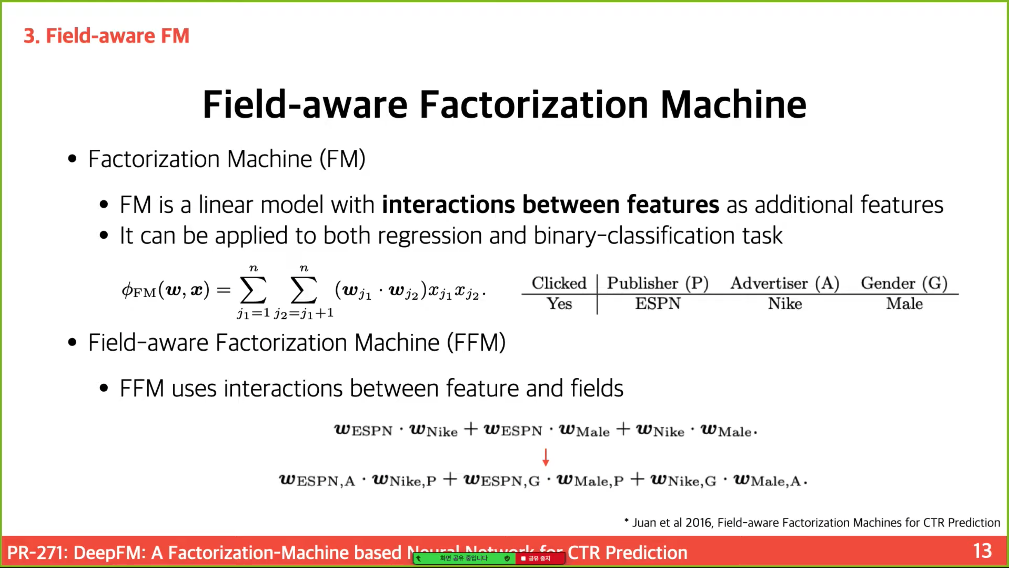
FM Component

FM(Feature machine) 모델은 (order-1) interaction 뿐 아니라 각 feature latent vectors의 inner product로 pairwise (order-2) interactions을 학습한다.
[특징]: weight 대신 V_i, V_j(latent vectors) 사용함
As Figure 2 shows, the output of FM is the summation of an Addition unit and a number of Inner Product units:
$y_{FM} = <w, x> + \Sigma^d_{j_1=1} \Sigma^d_{j_2=j_1+1} <V_i, V_j> x_{j_1}· x_{j_2},$ (2)
where $w ∈ R^d$ and $V_i ∈ R^k (k\ is\ given)^2$.
The Addition unit (<w, x>) reflects the importance of order-1 features, and the Inner Product units represent the impact of order-2 feature interactions.
- [참고] 참고 youtube 동영상에서 FFM(Field-aware Factorization Machine)으로 설명함
- 어떠한 Field와 interaction 하는지에 따라 Weight을 다르게 사용하여 학습한다.
- wide & deep과 다른점: linear로 하던 작업(cross product Transformation) → FM component 부분으로 변경함
Deep Component
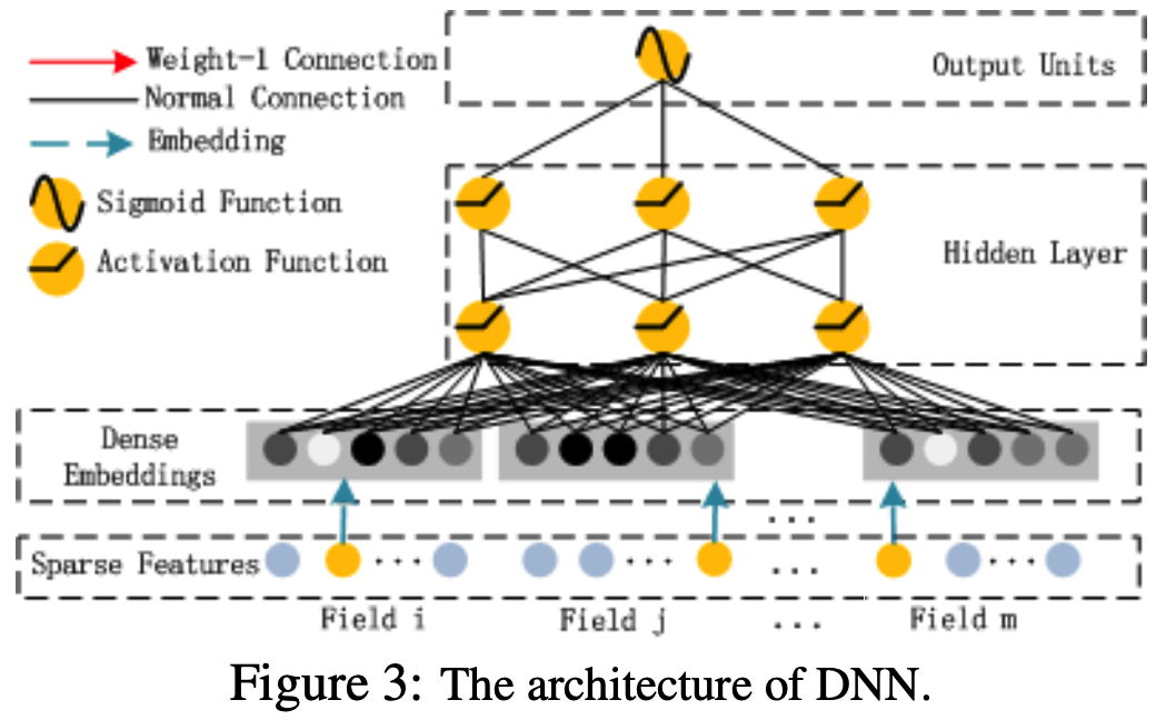
Deep Component는 high-order feature interactions를 학습하기 위한 feed-forward neural network이다.
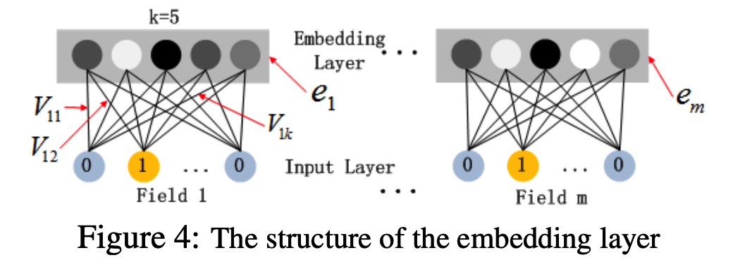
Figure 4 highlights the sub-network structure from the input layer to the embedding layer.
FM model을 통해 latent feature vectors를 학습하기 때문에 pre-training이 필요없어 end-to-end 학습이 가능하다.
Denote the output of the embedding layer as:
$a^{(0)} = [e_1, e_2, ..., e_m],$ (3)
where ei is the embedding of i-th field and m is the number of fields.
Then, a(0) is fed into the deep neural network, and the forward process is:
$a^{(l+1)} = σ(W^{(l)}a^{(l)} + b^{(l)}),$ (4)
where l is the layer depth and σ is an activation function. a(l), W(l), b(l)are the output, model weight, and bias of the l-th layer. (단순 FFN 식과 같음)
최종적으로 sigmoid function을 통과한 CTR prediction:
$y_{DNN} = σ(W^{(|H|+1)}· a^{(H)} + b^{(|H|+1)})$,
where |H| is the number of hidden layers. (논문에 누락?된 괄호 추가함)
We would like to point out the two interesting features of this network structure:
- while the lengths of different input field vectors can be different, their embeddings are of the same size (k);
- 보통 embedding layer의 특징임
- the latent feature vectors (V) in FM now server as network weights which are learned and used to compress the input field vectors to the embedding vectors.
- FM 먼저 훈련하는 것은 아니고 동시에 훈련(같이 사용한다)
2.2 Relationship with the other Neural Networks
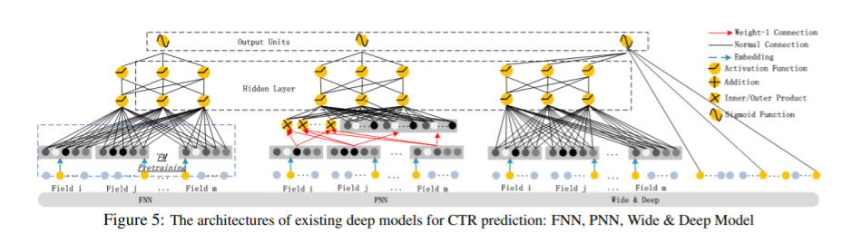
- FNN(Factorization-machine supported Neural Network)
- PNN(Product-based Neural Network)
- Wide & Deep Model
- [예시 참고] wide & deep model from Google
- Deep에서 훈련: 참새, 비둘기는 날 수 있어 -> 날개 달린 짐승은 날 수 있어
- Wide에서 훈련 : 펭귄 못 날아
- Source: https://ai.googleblog.com/2016/06/wide-deep-learning-better-together-with.html
The human brain is a sophisticated learning machine, forming rules by memorizing everyday events (“sparrows can fly” and “pigeons can fly”) and generalizing those learnings to apply to things we haven't seen before (“animals with wings can fly”). Perhaps more powerfully, memorization also allows us to further refine our generalized rules with exceptions (“penguins can't fly”).
Summarizations

: 네 가지 측면에서 다른 딥 모델과 비교해봤을 때, DeepFM은 pre-training과 feature engineering이 필요하지 않은 유일한 모델이며, low- and high-order feature interactions를 모두 capture한다.(Table 1)
[나머지 논문 참고]