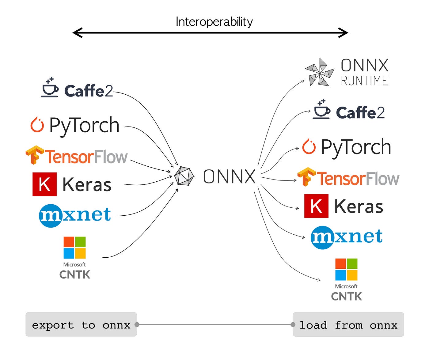
과거의 Tensorflow로 짜둔 모델을 Pytorch로 새롭게 훈련하지 않고 wegiht과 bias를 가져와서 변환을 해보고자 했습니다. (2022.07.05 기준) 아직 테스트는 진행하지 못함. 추후에 샘플 모델 변환 테스트를 진행 후 코드를 추가로 올리도록 하겠습니다. (2022.07.12 기준) Tensorflow -> ONNX -> Pytorch Test 완료
# from TensorFlow Model to PyTorch Model# tf_module의 weight를 torch_module의 weight에 적용하는 예시
tf_weights = tf_model.get_weights()[0]
tf_biases = tf_model.get_weights()[1]
## TF와 Torch의 weight shape이 다름 → Transpose 하기
torch_model.weight.data = torch.from_numpy(tf_weights)
torch_model.bias.data = torch.from_numpy(tf_biases)
  # from PyTorch Model to TensorFlow Model
  weight = torch_model.state_dict()["weight"].detach().numpy()
  bias = torch_model.state_dict()["bias"].detach().numpy()

  ## TF와 Torch의 weight shape이 다름 → Transpose 하기
  tf_model.set_weights([weight, bias])
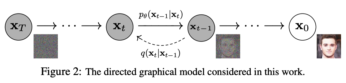
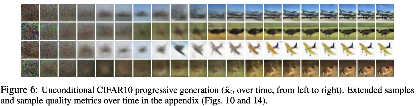
forward diffusion process q(xt|xt−1): noise를 점점 증가 시켜 가면서 학습 데이터를 특정한(Gaussian) noise distribution으로 변환
reverse generative process pθ(xt−1|xt): noise distribution으로부터 학습 데이터를 복원(=denoising)하는 것을 학습단 위과정을 Markov Chain으로 표현.
왜 잘될까?
기존의 AutoEncoder와 같은 모델의 경우 Encoder 부분에서 어느 정도로 data가 encoding이 될지 알 수 없고 조절할 수 없었지만 Diffusion 모델의 경우 각 time step 마다 약간의 noise가 추가되고 reverse할 때 그 지정된 만큼(?), 종류(?)의 noise를 복원해내면 되기 때문이지 않을까..(마치 작은 tasks로 쪼개서 문제를 해결해나가듯)
Langevin dynamics provides an MCMC procedure to sample from a distribution p(x) using only its score function ∇xlogp(x).
sθ≈∇xlogp(x)
[Using Langevin dynamics to sample from a mixture of two Gaussians.]
이 논문에서는 diffusion model의 샘플링 프로세스가 autoregressive 모델로 일반화가 가능하다는 것과 autoregressive의 decoding과 유사한 일종의 점진적 decoding이라는 것을 보여준다.
** autoregressive decoder: 과거의 자기 자신을 사용하여 현재의 자신을 예측하는 모델이다. (from wiki)
Xt=c+Σpi=1φiXt−1+εt
2. Background
Forward process(diffusion process: from data to noise)
diffusion model이 다른 유형의 latent 모델과 구별되는 것은 대략적인 사후 확률q(x_1:T|x0)이 데이터에 variance shedule β1,…,βT 에 따라 Gaussian noise를 점진적으로 추가하는 Markov Chain에 고정된다는 것이다.
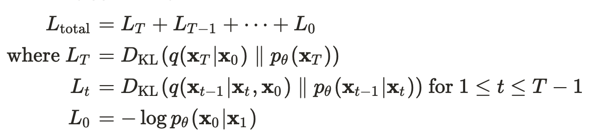
stochastic gradient descent으로 L의 random 항을 최적화함으로 효율적인 훈련이 가능하다. (Appendix A)
Loss_total
(모든 KL divergences는 Gaussian 분포들의 비교)
** KL divergences (from wiki)
: a measure of how one probability distribution P is different from a second, reference probability distribution Q.(=어떤 이상적인 분포에 대해, 그 분포를 근사하는 다른 분포를 사용해 샘플링을 한다면 발생할 수 있는 정보 엔트로피 차이를 계산한다.)
DKL(P||Q)=ΣP(x)log(P(x)Q(x))
** connections: Log likelihood, KL Divergence
The parameters that minimize the KL divergence are the same as the parameters that minimize the cross entropy and the negative log likelihood!
3. Diffusion models and denoising autoencoders
[detail은 논문 참고]
forward 프로세스의 분산 βt와 reverse 프로세스의 model architecture, Gaussian distribution parameterization(mu)을 선택해야한다.
Forward process: βt를 상수 취급(are fixed)하기 때문에 LT상수취급하여 훈련에서 무시
Reverse process (L1:T−1):
μθ를 평균 근사 훈련을 하여 ˜μt를 예측하거나 parameterization을 수정하여 ϵ을 예측하도록 훈련.
Data scaling (L0):(샘플링이 끝나면 μθ(x1,1) 를 noise를 제거하고 표시한다.)
0 ~ 255로 구성되어있는 이미지 데이터는 [−1,1]에서 선형 확장된다. 이렇게 하면 reverse process가 standard normal 사전분포 p(xT)에서 시작하여 일관되게 확장된 입력에 작동한다.
Simplified training objective
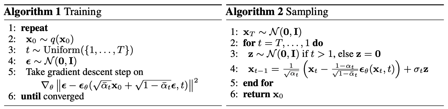
Algorithm 1, 단순화된 objective를 이용한 전체 training 프로세스
variational bound의 변형에 대해 학습하는 것이 sample 품질(구현 더 간단)에 더 유리하다는 것을 발견함:
Lsimple(θ):=Et,x0,ϵ[||ϵ−ϵθ(√ˉαx0+√1−ˉαtϵ,t)||2]
Algorithm 2, 전체 샘플링 프로세스는 데이터 밀도의 학습된 gradient로 θ를 사용하는 Langevin dynamics 과 유사하다. (ϵθis a function approximator intended to predict ϵ from xt)
4. Experiments
[Details are in Appendix B.]
Our neural network architecture follows the backbone of PixelCNN++ [52], which is a U-Net [48] based on a Wide ResNet [72].
We replaced weight normalization [49] with group normalization [66] to make the implementation simpler.
Our 32 × 32 models use four feature map resolutions (32 × 32 to 4 × 4), and our 256 × 256 models use six.
All models have two convolutional residual blocks per resolution level and self-attention blocks at the 16 × 16 resolution between the convolutional blocks [6].
Diffusion time t is specified by adding the Transformer sinusoidal position embedding [60] into each residual block.
Semi-supervised learning (SSL)은 labeld data와 unlabeled data 모두를 통합하는 기능이 있기 때문에 상당한 가치가 있다. Graph-based semi-supervised learning (GSSL)은 다양한 도메인에서 장점이 있다는 것이 입증되었다. 논문의 주요한 기여는 graph regularization과 graph embedding methods를 포함한 GSSL의 새로운 일반화 분류법에 있다.
1. Introduction
Graph-based SSL (GSSL)은 graph 구조상 중요한 manifold를 압축하여 반영하여 자연스럽게 사용될 수 있기때문에 특히 유망하다. graph는 구조적으로 nodes는 모든 samples를 표현할 수 있고 weighted edges는 nodes의 쌍 사이의 유사성을 반영한다.
[GSSL의 주요 과정]
Step 1. Graph construction.
A similarity graph는 labeled, unlabeled samples를 포함한 데이터로 구성되어있다.
original samples사이의 관계를 잘 표현하는 것이 중요한 과제이다.
Step 2. Label inference.
이전 step에서 만들어진 graph 구조 정보를 통합하여 labeled samples로 부터 unlabeled samples로 label 정보를 전파하는 것을 수행한다.
(this paper) Label inference methods are then categorized into two main groups: graph regularization methods and graph embedding methods. [논문참고]
image classification, natural language understanding 등 기존 tasks의 데이터는 Euclidean space에서 표현했다. 하지만 application 수가 증가하며 생성된 데이터는 non-Euclidean domains이고 이는 object 사이에 복잡한 관계를 갖는 graph로 표현된다.
1. Introduction
graphs는 불규칙적일 수 있다. 다양한 순서가 없는 node를 가질수도, node에 연결된 nieghbors의 숫자도 다를 수 있다. 따라서 graph domain에는 다르게 적용해야한다.
graph 데이터를 다루기위해 기존의 딥러닝 CNNs, RNNs, autoencoder 방법으로부터 새로운 일반화를 통한 응용한 연구가 진행되어왔다. 예를 들어 graph convolution은 2D convolution의 일반화가 될 수 있다. 2D convolution과 유사하지만 graph convolution은 node’s neighborhood 정보의 weight average를 가진다.
outlines the background of graph neural networks, lists commonly used notations, and defines graph-related concepts.
A. Background
A brief history of graph neural networks (GNNs)
이전 연구들은 recurrent graph neural networks의 카테고리였다. 고정된 point에 도달할때 까지 neighbor information을 전파하는 방법으로 target node’s representation을 학습한다. 하지만 이 프로세스는 컴퓨팅 비용이 비싸며 이 문제를 극복하기 위한 노력이 증가해왔다.
2009년에는 RNN(message passing)의 아이디어를 상속하면서 구조적으로 non-recursive layer를 합성하여 graph mutual dependency를 해결하는 RecGNNs(Micheli et al.) 방법이 제안되었다.
CV 도메인에서 CNN의 성공으로 graph를 데이터를 병렬적 개발하기 위한 convolution이 재정의되었다. ConvGCNNs(Bruna et al.(2013)) 은 spectral-based 접근법과 spatial-based 접근법으로 주요하게 나눠진다.
Graph neural networks vs. network embedding
network embedding의 목적은 low-dimensional vector로 representation을 생성하고 network topology structure와 node content information을 모두 보존하여 classification, clustering, recommendation등을 쉽게 수행할수 있도록 하는 것이다. matrix factorization, random walks 방법(non-deep learning method)을 사용한다. (예시, support vector machines for classification)
GNNs은 딥러닝 모델이며 end-to-end graph와 연관된 task를 해결하는 것이 목적이다. GNNs는 다양한 task를 위한 neural network model의 그룹이며 다양한 network embedding을 포함하고 있다.
Graph neural networks vs. graph kernel methods
GNNs과 유사하게 graph kernels는 mapping function을 이용하여 graphs or nodes를 vector space로 임베딩할 수 있다. mapping function이 learnable하기보다는 deterministic하다는 점이 다르다.
B. Definition
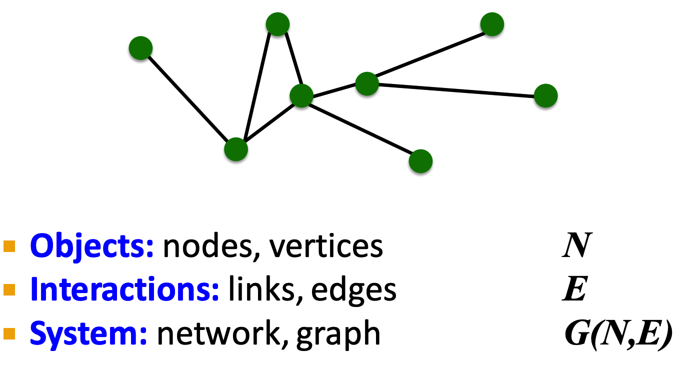
Definition 1 (Graph):
G=(V,E), V: nodes, E: set of edges
vi∈V,eij=(vi,vj)∈E
neighborhood of a nodeN(v)=u∈V|(v,u)∈E
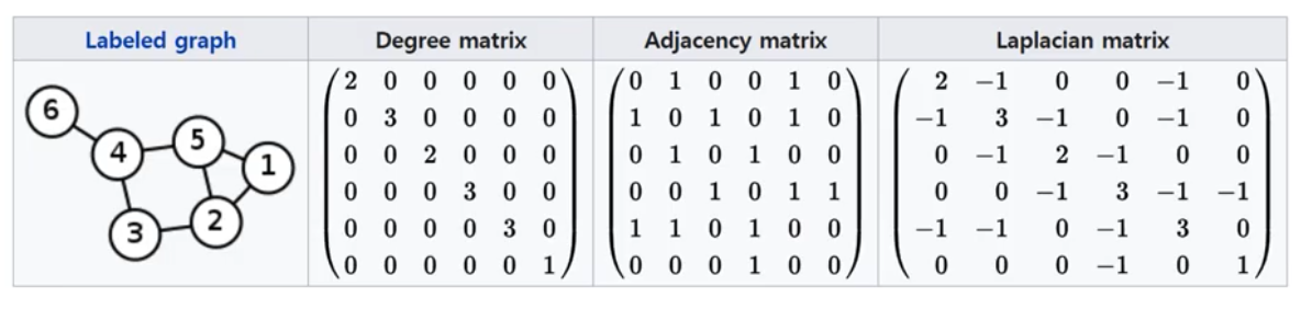
adjacency matrixA is n×n matrix
http://web.stanford.edu/class/cs224w/
** 인접 행렬: edges의 관계를 표현
{Aij=1,ifeij∈EAij=0,ifeij∉E
node attributes matrixX∈Rn×d
node feature attribute xv∈Rd
edge attributeXe∈Rm×c
edge feature attribute xev,u∈Rc
Definition 2 (Directed Graph):
directed(방향이 있는) graph는 node로부터 다른 node로 향하는 edges가 있는 것이다. adjacecy matrix가 대칭적인 경우에만 undirected graph이다.
spatial-temporal graph는 node attributes가 시간에 따라 dynamic하게 변화하는 attributed graph이다.
3. Categorization and Frameworks
clarifies the categorization of graph neural networks
A. Taxonomy of Graph Neural Netowrks (GNNs)
Recurrent graph neural networks (RecGNNs): GNN의 개척자라고 볼 수 있다.
RecGNN의 목적은 recurrent neural architectures로 node representation을 학습하는 것이다. graph의 node은 stable equilibrium(=변화하지 않는 안정된 상태)에 도달할 때까지 neighbor와 정보를 교환한다고 가정한다.
Convolutional graph neural networks (ConvGNNs): grid data로 부터 graph data로 convolution 연산을 일반화한다.
주된 아이디어는 feature xv 와 neighbors’ features xu(where u∈N(v))를 조합하여 node v’s features xu를 생성하는 것이다. RecGNNs와 달리 ConvGNNs는 high-level node representation을 추출하기 위해 multiple graph convolutional layers를 쌓는다.
Figure 2a shows a ConvGNN for node classification.
Figure 2b demonstrates a ConvGNN for graph classification.
Spatial-temporal graph neural networks (STGNNs): hidden patterns를 학습하는 것이 목적이다.
핵심 아이디어는 spatial dependency와 temporal dependency를 한번에 고려하는 것이다.
Figure 2d illustrates a STGNN for spatial-temporal graph forecasting.
B. Frameworks
mechanisms
Node-level outputs relate to node regression and node classification tasks. With a multi-perceptron or a softmax layer as the output layer, GNNs are able to perform node-level tasks in an end-to-end manner.
Edge-level outputs relate to the edge classification and link prediction tasks. two nodes’ hidden representations로 the label/connection strength of an edge 예측할 수 있다.
Graph-level outputs relate to the graph classification task. graph level에서 compact representation를 얻을 수 있다.
Training Frameworks
Many GNNs (e.g., ConvGNNs) can be trained in a (semi-) supervised or purely unsupervised way within an end-to-end learning framework, depending on the learning tasks and label information available at hand.
Semi-supervised learning for node-level classification
Supervised learning for graph-level classification