AN IMAGE IS WORTH 16X16 WORDS: TRANSFORMERS FOR IMAGE RECOGNITION AT SCALE

• 논문
  • https://arxiv.org/pdf/2010.11929.pdf
• code
  • https://github.com/google-research/vision_transformer
• 참고
  • https://www.youtube.com/watch?v=TrdevFK_am4

** 아래의 내용과 이미지는 위의 논문을 기반으로 작성하였습니다.

** 수정할 부분이나 의견이 있다면 댓글로 달아주세요~

ABSTRACT

Transfomer architecture는 NLP task에서 공공연히 standard한 모델이 되어왔지만 CV(Computer Vision) task에서는 여전히 한계가 있다.

우리는 CNN을 사용할 필요없이 image를 sequcese of patches로 직접 적용하는 transformer 모델 자체가 classification task에서 좋은 성능을 보인다는 것을 보여준다.

대량의 data를 pre-trained하고 multiple mid-sized or small images를 banchmarks (ImageNet, CIFAR-100, VTAB, etc.)로 transferred할 때 ViT는 적은 computational resource를 사용하여 훈련하여도 SOTA와 비교해도 좋은 결과를 얻을 수 있다.

1 INTORDUCTION

Transformer(Self-attention-based architectures)가 large dataset으로 훈련된 pre-trained모델로 NLP task에서 많이 채택되고 있다.

CV에서는 CNN을 사용하는 경우가 여전히 우세하다. attention aptterns을 사용할 때 여러 test가 있었지만 아직 충분히 scaled dffectively 모델이 없다.

우리는 image를 잘라서 patches(treated the same way as tokens (words))로 만들고 sequence를 linear ebedding로 만들어 transformer에 넣었다. ViT는 충분한 scale로 pre-trained하고 fewer datapoints로 task를 trasnferred할때 상당히 좋은 결과를 달성할 수 있다.

2 RELATED WORK

Naive application of self-attention to images would require that each pixel attends to every other pixel. With quadratic cost in the number of pixels, this does not scale to realistic input sizes. Thus, to apply Transformers in the context of image processing, several approximations have been tried in the past.

Many of these specialized attention architectures demonstrate promising results on computer vision tasks, but require complex engineering to be implemented efficiently on hardware accelerators.

Most related to ours is the model of Cordonnier et al. (2020), which extracts patches of size 2 × 2 from the input image and applies full self-attention on top. This model is very similar to ViT, but our work goes further to demonstrate that large scale pre-training makes vanilla transformers competitive with (or even better than) state-of-the-art CNNs. Moreover, Cordonnier et al. (2020) use a small patch size of 2 × 2 pixels, which makes the model applicable only to small-resolution images, while we handle medium-resolution images as well.

We focus on these two latter(ImageNet-21k and JFT-300M) datasets as well, but train Transformers instead of ResNet-based models used in prior works.

3 METHOD

In model design we follow the original Transformer (Vaswani et al., 2017) as closely as possible. An advantage of this intentionally simple setup is that scalable NLP Transformer architectures – and their efficient implementations – can be used almost out of the box.

3.1 VISION TRANSFORMER (ViT)

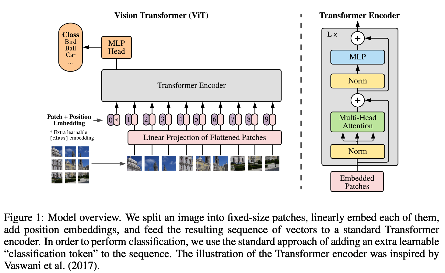
standard Transformer는 input으로 1D sequnce of token embeddings을 가지기 때문에 2D images를 다루기 위해 patches(이미지를 자른 것)를 flatten하고 trainable linear projection을 사용하여 D 차원에 mapping한다.

potision embeddings(1D)는 위치 정보를 유지하기 위해 patch embeddings에 합산한다. sequence of embedding vectors는 encoder의 입력으로 사용된다.

• linear projection (Eq. 1).the patch embedding projection E (Eq. 1) is applied to patches extracted from a CNN feature map.
  • $z_0 = [x_{class}; x^1_pE;x^2_pE; ...;x^N_pE] + E_{pos}, E \in \mathbb{R}^{(P^2C) \times D}, E_{pos} \in \mathbb{R}^{(N+1)\times D}$

BERT의 [class] token과 비슷하게, (Transformer encoder $(z^0_L)$ 의 output 상태가 image representation y 역할을 하는) sequnce of embedded patches 앞에 learnable embedding을 추가한다.

• (Eq.4)
  • $y = LN(z^0_L)$ , Layernorm (LN)

Transformer Encoder는 Multihead self-attention(MSA) 과 MLP block (Eq. 2, 3)의 layers로 구성된다. Layernorm (LN)은 모든 block 이전에 적용되고 residual connection (+ 기호 사용)은 모든 block 이후에 적용된다.

• (Eq.2)Multihead self-attention(MSA) is an extension of SA in which we run k self-attention operations, called “heads”, in parallel, and project their concatenated outputs. (in Appendix A)
  • $z'l = MSA(LN(z{l-1})) + z_{l-1}$ $l = 1 ... L$
• (Eq.3)MLP에는 2개의 GELU layers 사용
  • *참고: Gaussian Error Linear Units (GELUs) is an activation function. (non-linear) https://paperswithcode.com/method/gelu
  • $z_l = MLP(LN(z'_l)) + z'_l$ $l = 1 ... L$

Inductive bias.

CNN에서는 locality, 2D neighborhood structure, and translation equivariance가 전체 모델을 통해 각 layer로 다시 들어간다.

ViT에서는 MLP layers만 local and translationally equivariant이고, self-attention layers는 global이다.

Hybrid Architecture.

hybrid model에서는 patch embedding projection E(Eq. 1)에 CNN feature map으로 부터 추출된 patches가 적용된다. 특별한 경우로, patches는 spatial size 1x1 가질수 있다. input sequence는 단순히 spatial dimensions of the feature map을 flattening하고 Transformer dimesion을 projecting하여 얻는다. ( Abstract 에서는 CNN 필요없다고 했지만...)

3.2 FINE-TUNING AND HIGHER RESOLUTION

일반적으로 대규모 데이터셋에 대해 ViT를 pre-train하고 (smaller) downstream task로 fine-tune한다. 이를 위해 pre-trained prediction head를 제거하고 zero-initialize된 DxK(K: the number of downstream classes) feedforward layer를 연결한다. 종종 higer resolution으로 fine-tune하는 것이 도움이 된다.

hider resolution을 사용할 때는 patch size를 같게 유지하기 때문에 effective sequence length가 커진다. ViT는 임의의 sequence length를 처리할 수 있지만 pre-trained position embeddings가 더 이상 의미가 없을 수 있다. 따라서 원본에서 location에 따라 pre-trained position embeddings의 2D interpolation을 수행한다. (수동으로 bias 넣음)

4 EXPERIMENTS

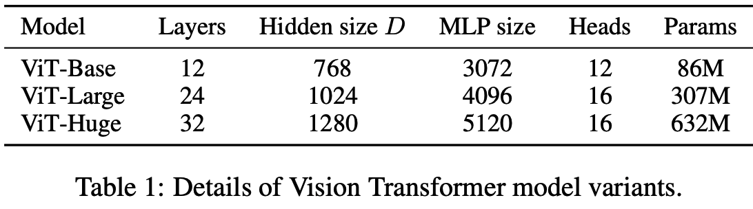
ViT-L/16 means the “Large” variant with 16×16 input patch size.

Note that the Transformer’s sequence length is inversely proportional to the square of the patch size, thus models with smaller patch size are computationally more expensive.

Globally, we find that the model attends to image regions that are semantically relevant for classification (Figure 6).

5 CONCLUSION

image recognition을 Transformers에 직접 적용해보았다. 기존 computer vision에서 self-attention을 사용하는 방법과 달리, 이 논문에서는 image를 a sequence of patches로서 NLP에서 사용되는 standard Transformer encoder로 처리한다.

• Challenges
  1. 다른 CV task(detection and segmentation)에 ViT 적용하기
  2. self-supervised pre-training 방법 탐색하기

나의 결론

• 최근 동향을 보면, Transformer는 CNN, LSTM 과 같은 general deep learning model이 되었다. 오히려 NLP, CV 등 task에 국한되지 않고 대체적으로 (SOTA에 준하는 혹은 뛰어넘는) 좋은 성능을 보이고 있다. (nlp와 달리 image는 local&global(position) feature(information)가 중요함)
• 이 논문에서는 image input을 transformer model에 어떻게 넣어야 효과적일까? 에 대한 방법을 소개한다.
  • 방법요약: patch로 이미지를 잘라서(or CNN으로 feature map 생성해서-hybrid architecture) 1dim으로 flatten 시키고 (Transformer가 1d를 input으로 받음) 각 patch별로 position embedding을 붙여서 transformer에 넣는다. (idea는 단순함)
    • 아래 이미지 Source: https://www.youtube.com/watch?v=QkwNdgXcfkg
    
  • 다만, 데이터셋이 적으면 train 하기 어려움 → (google에서 ViT를 large dataset으로 pre-train함) fine-tuning(transferred learning)해서 사용하면 좋은 성능 기대할 수 있음

오늘은 딥러닝 모델을 생성할 때 많이 사용하는 Python 라이브러리 중 Tensorflow의 기본 동작 원리와 코드, Tensorflow 2.0에서는 어떻게 변화하였는지에 대해 살펴보도록 하겠습니다!

텐서플로 1 코드를 텐서플로 2로 바꿔보자

• Source:https://www.tensorflow.org/guide/effective_tf2
• https://www.tensorflow.org/guide/migrate

여전히 텐서플로 1.X 버전의 코드를 수정하지 않고 텐서플로 2.0에서 실행할 수 있습니다(contrib 모듈은 제외):

import tensorflow.compat.v1 as tf
tf.disable_v2_behavior()

→ contrib 모듈의 경우 각 함수에 맞게 대체 가능한 모듈 찾아서 변경하기 (이 부분이 조금 귀찮음)

텐서플로 1 vs 2 동작원리 살펴보기

1. 텐서플로 1.x 코드

import tensorflow as tf  # v1

# 1. tf.placeholder를 사용하여 그래프에 입력할 값의 형태를 미리 지정한다.
in_a = tf.placeholder(dtype=tf.float32, shape=(2))
in_b = tf.placeholder(dtype=tf.float32, shape=(2))

# 2. 그래프 생성
def forward(x):
    # tf.get_variable을 사용하여 변수를 생성하고 tf.variable scope로 그 범위를 지정한다.
    with tf.variable_scope("matmul", reuse=tf.AUTO_REUSE):
        W = tf.get_variable("W", initializer=tf.ones(shape=(2,2)),
                            regularizer=tf.contrib.layers.l2_regularizer(0.04))
        b = tf.get_variable("b", initializer=tf.zeros(shape=(2)))
        return W * x + b

out_a = forward(in_a)
out_b = forward(in_b)

reg_loss = tf.losses.get_regularization_loss(scope="matmul")

# 3. tf.Session.run을 이용하여 그래프를 실행한다.
# The value returned by run() has the same shape as the fetches argument.
# feed_dict을 이용하여 placeholder의 실제 입력값을 넣는다.
with tf.Session() as sess:
    sess.run(tf.global_variables_initializer())
    outs = sess.run([out_a, out_b, reg_loss],  # fetches
                    feed_dict={in_a: [1, 0], in_b: [0, 1]})

2. 텐서플로 2.x 코드로 변경

import tensorflow as tf  # v2

# tf.variable_scope 사용하지 않음
W = tf.Variable(tf.ones(shape=(2,2)), name="W")
b = tf.Variable(tf.zeros(shape=(2)), name="b")

@tf.function
def forward(x):	
    return W * x + b

# tf.placeholder & tf.Session.run를 사용하지 않음
# Session.run 대신 실제 입력값의 단순 함수 호출로 변경(즉시 실행가능)
out_a = forward([1,0])
out_b = forward([0,1])

regularizer = tf.keras.regularizers.l2(0.04)
reg_loss = regularizer(W)

: TensorFlow 2 패키지에는 pip 버전 >19.0이 필요합니다. (https://www.tensorflow.org/install)

결론

source: https://www.tensorflow.org/guide/migrate#결론

전체적인 과정은 다음과 같습니다:

1. 업그레이드 스크립트를 실행하세요.
2. contrib 모듈을 삭제하세요.
3. 모델을 객체 지향 스타일(케라스)로 바꾸세요.
4. 가능한 **[tf.keras](<https://www.tensorflow.org/api_docs/python/tf/keras>)**나 **[tf.estimator](<https://www.tensorflow.org/api_docs/python/tf/estimator>)**의 훈련과 평가 루프를 사용하세요.
5. 그렇지 않으면 사용자 정의 루프를 사용하세요. 세션과 컬렉션은 사용하지 말아야 합니다.

텐서플로 2.0 스타일로 코드를 바꾸려면 약간의 작업이 필요하지만 다음과 같은 장점을 얻을 수 있습니다:

• 코드 라인이 줄어 듭니다.
• 명료하고 단순해집니다.
• 디버깅이 쉬워집니다.

텐서플로 2 | Basic Model 만들어보자

→ tensorflow2라고 쓰고 tf.keras 라고 읽는다.

참고: https://www.tensorflow.org/guide/keras

• 아래의 tensorflow2 모델은 이미지 분류를 예시로 작성하였습니다.

1. dataset 생성하기

• 여러 방법이 있지만 2가지만 소개합니다.

import tensorflow as tf

# Case 1
## ex, 
## x_train = [train_data_dir/file1.jpg, train_data_dir/file2.jpg, train_data_dir/file3.jpg, ...]
## y_train = [class1, class1, class2, ...]

train_dataset = tf.data.Dataset.from_tensor_slices((x_train, y_train))

# 필요에 따라 map_func 사용할 수 있음 (ex, 이미지 read, resize, ...)
train_dataset = train_dataset.map(lambda item1, item2: tf.numpy_function(
                                      map_func, [item1, item2], [tf.float32, tf.float32]))

# Shuffle and batch
train_dataset = train_dataset.shuffle(BUFFER_SIZE, seed=2021).batch(BATCH_SIZE)
train_dataset = train_dataset.prefetch(BUFFER_SIZE//2)

# Case 2
## ex, train_data_dir/class1/file1.jpg, train_data_dir/class1/file2.jpg, train_data_dir/class2/file3.jpg, ...
train_dataset = tf.keras.preprocessing.image_dataset_from_directory(train_data_dir,
                                                                    seed=2021,
                                                                    image_size=(img_height, img_width),
                                                                    batch_size=batch_size)

# class name 찾을 수 있음
class_names = train_dataset.class_names

train_dataset = train_dataset.cache().prefetch(BUFFER_SIZE//2)

2. model 생성하기

2.1 함수형

• 함수형 API 가이드
• https://www.tensorflow.org/guide/keras/functional

import tensorflow as tf
class_num = 5

def create_image_classification_model(input_shape):
    # 아래의 구조의 경우, tf.keras.Model 대신 tf.keras.models.Sequential 사용 가능
    # 다만, 다중 입력 및 출력, residual connection, attention 등 Model function이 활용성이 더 높음
    model_input = tf.keras.Input(shape=input_shape)

    embedding = tf.keras.layers.Conv2D(2, 3, padding='same', activation='relu')(model_input)

    embedding = tf.keras.layers.GlobalAveragePooling2D()(embedding)

    embedding = tf.keras.layers.Dense(128, activation='relu')(embedding)
    embedding = tf.keras.layers.Dropout(0.2)(embedding)
    
    embedding = tf.keras.layers.Dense(class_num, activation='softmax', name='output')(embedding)
    
    return tf.keras.Model(model_input, embedding, name='image_classification_model')

input_shape = (256, 256, 3)
classification_model = create_image_classification_model(input_shape)

## sample test
temp_input = tf.random.uniform(input_shape, dtype=tf.float32, minval=0, maxval=256)
output = classification_model.predict(tf.expand_dims(temp_input, 0))
output.shape  # (1, 5)

# model architecture(shape) & params 확인
classification_model.summary()

## (구조가 더 복잡한 경우,) model architecture(shape) ploting하여 확인 가능
# tf.keras.utils.plot_model(classification_model, "image_classification_model.png", show_shapes=True)

2.2 클래스 상속

• 모델 subclassing API 가이드
• https://www.tensorflow.org/guide/keras/custom_layers_and_models

import tensorflow as tf
class_num = 5

class ClassificationModel(tf.keras.Model):
    def __init__(self, class_num, dim=128, rate=0.1):
        super(ClassificationModel, self).__init__()
        self.conv2d = tf.keras.layers.Conv2D(2, 3, padding='same', activation='relu')
        
        self.dense1 = tf.keras.layers.Dense(dim, activation='relu')
        self.dense2 = tf.keras.layers.Dense(class_num, activation='softmax', name='output')
        
        self.gapooling = tf.keras.layers.GlobalAveragePooling2D()
        self.dropout = tf.keras.layers.Dropout(rate)
        

    def call(self, inputs):

        embedding = self.conv2d(inputs)

        embedding = self.gapooling(embedding)

        embedding = self.dense1(embedding)
        embedding = self.dropout(embedding)

        embedding = self.dense2(embedding)

        return embedding


input_shape = (256, 256, 3)
classification_model = ClassificationModel(class_num=class_num, rate=0.2)

## sample test
temp_input = tf.random.uniform(input_shape, dtype=tf.float32, minval=0, maxval=256)
output = classification_model(tf.expand_dims(temp_input, 0))

output.shape # TensorShape([1, 5])

# model architecture & params 확인
classification_model.build((None, 256, 256, 3))
classification_model.summary()

3. model 훈련하기

classification_model.compile(optimizer='adam',
                             loss=tf.keras.losses.CategoricalCrossentropy(from_logits=False),
                             metrics=['categorical_accuracy'])

history = classification_model.fit(train_dataset,
                                   epochs=EPOCHS,
                                   validation_data=val_dataset,
                                   callbacks=[modelcheck],)  # callbacks: modelcheckpoint, etc

• 시각화하기

  import matplotlib.pyplot as plt
  
  acc = history.history['accuracy']
  val_acc = history.history['val_accuracy']
  
  loss=history.history['loss']
  val_loss=history.history['val_loss']
  
  epochs_range = range(EPOCHS)
  
  plt.figure(figsize=(8, 8))
  plt.subplot(1, 2, 1)
  plt.plot(epochs_range, acc, label='Training Accuracy')
  plt.plot(epochs_range, val_acc, label='Validation Accuracy')
  plt.legend(loc='lower right')
  plt.title('Training and Validation Accuracy')
  
  plt.subplot(1, 2, 2)
  plt.plot(epochs_range, loss, label='Training Loss')
  plt.plot(epochs_range, val_loss, label='Validation Loss')
  plt.legend(loc='upper right')
  plt.title('Training and Validation Loss')
  plt.show()​

  source: https://www.tensorflow.org/tutorials/images/classification

4. model save & load, predict 하기

model_save_path = 'image_classification_model'

# model architecture & weight 저장
classification_model.save(model_save_path)

# model architecture & weight 불러오기
new_model = tf.keras.models.load_model(model_save_path)
# new_model.trainable = False  # transfer learning시 pre-trained model을 freezing할 때 사용, layer별로 설정 가능

# 불러온 모델 predict
y_pred = new_model.predict(test_dataset,
                           steps=STEP_SIZE_TEST
                           )

• 논문
  
  • https://arxiv.org/pdf/2004.00049.pdf
• code
  • https://genforce.github.io/idinvert/

** 아래의 내용과 이미지는 위의 논문을 기반으로 작성하였습니다.

** 수정할 부분이나 의견이 있다면 댓글로 달아주세요~

[참고] 미리보기

• Source: https://www.youtube.com/watch?v=TVSJO9uNq7g

GAN Inversion : GAN을 거꾸로 하는 것

: real image를 latent space의 적절한 latent code로 Inversion하는 task

→ latent space를 배운다. (explainable)

⇒ latent space 상의 각각의 latent code로 부터 realistic한 image를 얻을 수 있다.

StyleGAN: 각 layer 마다 hierarchical latent code를 부여하여 generation

: 위의 구조는 realistic한 output을 얻을 수 있을뿐만 아니라 각 layer별로 latent vector의 의미가 다르게 훈련됨 → output 이미지를 조절할 수 있다.

Abstract

기존 GAN의 경우 real image를 editing하기위한 semantics를 배우기 어려웠다.

현존하는 inversion methods는 pixel 기준으로 target image를 reconstucting(재구성)하기 때문에 original latent space에 semantic한 inverted code를 배치시키는데 실패했다.

논문에서는 이러한 문제를 해결하기 위해 in-domain GAN inversion방식을 제안한다. input image를 reconstuct할 뿐아니라 image editing을 위한 semantically meaningful latent code로 invert할 수 있다.

→ in domain ( latent space 안에서) GAN inversion을 제시, real image에 semantic한 editing할 수 있다.

1 Introduction

• in domain 예: like face, tower, bedroom
• semantic 예 : eyeglasses, smile (→ face에서 자연스럽게?)

GAN은 image를 생성하는 generator와 실제 이미지와 가짜 이미지를 판별하는 discriminator로 구성되어있다.

최근 연구에서 GAN이 latnet space에서 풍부한 semantics를 encoding하는 방법으로 학습하고 latent code를 변경하면 output image에서 해당하는 attributes를 조작(manipulation)할 수 있다는 것을 보여줬다.

하지만, real image를 입력으로 사용하여 latent code를 추론하는 기능이 없기 때문에 이러한 manipulation을 적용하기에는 여전히 어렵다.

GAN Inversion으로 image sapce를 latent space로 mapping하여 generation process로 되돌리려는 시도가 많이 있지만, 기존 방법은 주로 input image의 pixel을 기준으로 reconstruct하는 것에 중점을 두었다.

하지만 이 논문에서는 GAN Inversion 작업에서 pixel 수준 뿐 아니라 latent space에 encoding된 semantic knoledge와 align되어야한다고 주장한다. 이런 semantically meaningful codes는 GAN이 학습한 domain에 종속되기 때문에 in-domian code라고 부른다.

2 In-Domain GAN Inversion

GAN Invert할 때 input image의 pixel값을 복구하는 것 외에도 inverted code가 semantically 의미있는지 여부도 고려한다.

여기서 semantics는 GAN이 관찰된 data로부터 학습한 emergent knoledge를 의미한다.

방법: as shown in Fig.2.

1. novel domain-guided encoder를 훈련하여 encoder에서 생성된 모든 code가 domain내에 있도록 image space를 latent space에 매핑한다.
2. inverted code의 semantic property에 영향을 주지않고 pixel 값을 더 잘 reconstruct하기위해 instance-level domain-regularized optimization한다.

Problem Statement.

GAN model은 generator G(·) : Z → X 와 discriminator D(·) 로 구성되어있다. GAN Inversion은 주어진 실제 이미지 x real을 복구하기 위해 최상의 잠복 코드 z inv를 찾는 reverse mapping of G(·)을 학습한다.

Choice of Latent Space.

일반적으로 GAN은 미리 정의된 distribution space (such as normal distibution) Z에서 latent code z를 샘플링한다.

최근 StyleGAN 모델은 Multi-Layer Perceptron (MLP)를 이용하여 initial latent space Z를 두번째 latent space W에 매핑한다음 w ∈ W를 Generator에 사용하는 (additional mapping) 방법을 제안했다. → GAN inversion task에서 많이 사용됨

3가지 이유로 이 논문에서도 inversion space로 W space를 선택한다.

(i) We focus on the semantic (i.e., in-domain) property of the inverted codes, making W space more appropriate for analysis.

(ii) Inverting to W space achieves better performance than Z space [35].

( but our approach can be performed on the Z space as well. For simplicity, we use z to denote the latent code in the following sections. )

(iii) It is easy to introduce the W space to any GAN model by simply learning an extra MLP ahead of the generator.

2.1 Domain-Guided Encoder

Fig.2(a)의 위에 있는 (conventional encoder)를 보면, latent codes $z^{sam}$는 랜덤하게 샘플링되어 Generator에 들어가고 연관된 synthesis $x^{syn}$ 이미지를 얻는다.

그리고 Encoder는 $x^{syn}$ 를 input으로 $z^{sam}$ supervisions으로 하고 eq1으로 훈련된다.

$min_{\Theta_E}L_E = ||z^{sam} - E(G(z^{sam}))||_2$, (1)

where $||·||_2$ denotes the $l_2$ distance and $\Theta_E$ represents the parameters of the encoder E(·).

→ it is not powerful enough to train an accurate encoder and cannot provide its domain knowledge

이러한 문제를 해결하기위해 저자는 domain-guided encoder(in the bottom row of Fig.2(a))를 제안한다.

→ 기존 gan 방법과 달리 latent space가 아닌 real image space에서 input image를 reconstruct 함 : G(E(xreal))

1. The output of the encoder is fed into the generator to reconstruct the input image such that the objective function comes from the image space instead of latent space.
2. Instead of being trained with synthesized images, the domain-guided encoder is trained with real images, making our encoder more applicable to real applications.
3. To make sure the reconstructed image is realistic enough, we employ the discriminator to compete with the encoder. (both two components of GAN are used).

이 방식으로 GAN 모델에서 최대한 많은 정보를 얻을 수 있다.

The training process can be formulated as LE, LD

$$min_{\Theta_E}L_E = ||x^{real}-G(E(x^{real}))||2 \\ + \lambda{vgg} ||F(x^{real}) - F(G(E(x^{real})))||2 \\ - \lambda{adv} \mathbb{E}{x^{real} \sim P{data}}[D(G(E(x^{real})))],$$ (2)

• loss1: per pixel loss
  • $||x^{real}-G(E(x^{real}))||_2$ : x와 (x >> Encoder >> generator >>) z를 비교하는 loss,
• loss2: perceptual loss
  • F(·) denotes the VGG feature extraction model.
    • perceptual loss: Perceptual loss란 [11]에서 처음으로 제안된 손실 함수로 입력과 GT를 미리 학습해 놓은 다른 딥러 닝 기반의 영상 분류 네트워크에 통과 시킨 후 얻 은 feature map 사이의 손실을 최소화 하는 방향 으로 필터 파라미터를 학습한다.
    • source: http://www.kibme.org/resources/journal/20200504094149078.pdf
  • $\lambda_{vgg} ||F(x^{real}) - F(G(E(x^{real})))||_2$ : vgg loss 사용
• loss3: discriminator loss
  • Pdata denotes the distribution of real data
  • $\lambda_{adv} \mathbb{E}{x^{real} \sim P{data}}[D(G(E(x^{real})))]$ : discriminator를 training용

$$min_{\Theta_D} L_D = \mathbb{E}{x^{real} \sim P{data}}[D(G(E(x^{real})))] \\ - \mathbb{E}{x^{real} \sim P{data}}[D(x^{real})] \\ + \frac{\gamma}{2} \mathbb{E}{x^{real} \sim P{data}} [|| \nabla_x D(x^{real})||_2^2],$$ (3)

• loss 1: discriminator loss
  • $\mathbb{E}{x^{real} \sim P{data}}[D(G(E(x^{real})))] - \mathbb{E}{x^{real} \sim P{data}}[D(x^{real})]$ : 가짜(생성된 이미지), real image discriminator loss
• loss 2: gradient regularization
  • $\frac{\gamma}{2} \mathbb{E}{x^{real} \sim P{data}} [|| \nabla_x D(x^{real})||_2^2]$ : 변화량에 penalty
  • γ is the hyper-parameter

2.2 Domain-Regularized Optimization

distribution level에서 mapping을 학습하는 GAN의 generation process와 달리, GAN inversion은 주어진 개별 image를 가장 잘 reconstruct하는 instance-level task와 비슷하다.

이러한 관점에서 볼때 encoder 만으로는 representation capability이 제한되어 완벽한 reverse mapping을 학습하기 어렵다. 따라서, 여전히 code를 pixel 값에서 개별 target image와 더 잘 fit하게 수정해야한다.

The top row of Fig.2(b)에서 latent code는 generator만을 기반으로 'freely' 최적화된다.

이것은 latent code를 제약이 없기때문에 an out-of-domain inversion이 발생할 가능성이 매우 높다.

The bottom of Fig.2(b)에서 보이는 것처럼, 2가지 개선사항으로 domain-regularized optimization을 설계한다.

1. We use the output of the domain-guided encoder as an ideal starting point which avoids the code from getting stuck at a local minimum and also significantly shortens the optimization process.
2. We include the domain-guided encoder as a regularizer to preserve the latent code within the semantic domain of the generator.

To summarize, the objective function for optimization is

$$z^{inv} = argmin_z (||x - G(z)||2 \\+ \lambda{vgg}||F(x) - F(G(x))||2 \\+ \lambda{dom}||z-E(G(z))||_2),$$ (4)

• x is the target image to invert
• λvgg : the perceptual loss
• λdom: encoder regularizer respectively
  
  • $\lambda_{dom}||z-E(G(z))||_2$
  • z와 (z >> Generator >> Encoder >>) z' 을 같도록 훈련 ⇒ semantic 의미를 잘 갖추도록 (z를 이미 잘 구해놓았다는 전제하고 z를 fine-tuning, 최적화)

3 Experiments

[논문 참고]

4 Discussion and Conclusion

in domain으로 훈련해서 out of distribution에서는 별로다.(in Fig.10) → semantic한 훈련이 되었다는 의미로 볼 수 있다.

결론적으로, in-domain inversion은 pixel level과 semantic level 모두에서 대상 이미지를 복구하는 데 가장 적합한 (latent) code를 찾는 것을 목표로 하며 real image editing을 상당히 용이하게 한다.

[논문] arxiv.org/pdf/1703.04247.pdf

** 아래의 내용은 위의 논문을 기반으로 재해석한 내용입니다.
** 오타 혹은 부족한 부분이 있다면 첨언 및 조언 환영합니다!

[참고] 미리보기

1. CTR(click-through rate): 정의

클릭률(CTR)은 광고를 본 사용자가 해당 광고를 클릭하는 빈도의 비율입니다. 클릭률(CTR)을 사용하면 키워드와 광고, 무료 제품 목록의 실적을 파악할 수 있습니다.

• CTR은 광고가 클릭된 횟수를 광고가 게재된 횟수로 나눈 값입니다(클릭수 ÷ 노출수 = CTR)

Source: https://support.google.com/google-ads/answer/2615875?hl=ko

2. Factorization Machine

FM은 매트릭스 요소화(Matrix factorization)를 통해 문제의 치수(dimension)를 줄이는 기능에서 이름을 얻습니다.

Factorization Machine은 분류 또는 회귀에 사용될 수 있으며 선형 회귀와 같은 기존의 알고리즘보다 대형 스파스(sparse) 데이터셋에서 훨씬 더 효율적입니다.

Source: https://www.megazone.com/techblog_180709_movie-recommender-with-factorization-machines/

Abstract

추천 시스템에서 CTR을 최대화하는 것은 매우 중요하다.

하지만 기존의 방법은 lower- 혹은 high order 둘 중 하나에만 적용할 수 있었다.

따라서 이 논문에서는 lower-와 high order 의 interaction을 고려하며 feature engineering이 필요없는 end-to-end 학습 모델인 DeepFM을 제안한다.

• [참고] 'Feature engineering이 필요없다'는 것을 강조하는 이유:
  • Source: https://youtu.be/zxXRGhSQ1f4?t=628
  • CTR prediction에서는 어떠한 모델을 쓰는지 만큼이나 어떠한 feature를 어떻게 넣을지, feature engineering이 매우 중요하다. (도메인에 따라 달라지기 때문에)

1 Intoduction

CTR 예측은 user가 추천 item을 클릭할 확률을 추정하는 것으로 사용자에게 반환될 item rank 선정과 revenue 개선 측면에서 매우 중요하다.

CTR 예측은 사용자의 click 행동 뒤에있는 암시적 feature interactions를 학습하는 것이 중요하다.

예를 들어,

1. 식사시간에 배달앱을 다운로드하는 경우가 많다. → "app category"와 "time-stamp"의 interaction (order-2)
2. shooting games & RPG games를 좋아하는 남자 청소년 → "app category"와 "gender"와 "age"의 interaction (order-3)
3. (고전 연관 규칙) 기저귀를 사는 사람들이 맥주도 같이 사더라 → "diaper"와 "beer"의 interaction (order-2)

하지만 대부분의 feature interactions는 3번 예시처럼 숨겨져 있어 machine learning을 통해서만 자동으로 capture될 수 있다.

Our main contributions are summarized as follows:

• FM(Factorization Machines)과 DNN(Deep Neural Networks)를 통합한 DeepFM(Figure 1)을 제안한다.
  • FM으로 lower-order feature interaction을 학습하고, DNN으로 high-order feature interaction을 학습한다.
• wide & deep model [Cheng et al., 2016] 모델과 다른점은 feature engineering 없이 end-to-end 학습을 하며, wide part와 deep part의 input과 embedding vector를 공유하기 때문에 더 효율적이다.

2 Our Approach

training data set이 n개의 (χ, y) instances로 구성되어있다고 가정한다. 여기서 x는 user와 item을 한 쌍(a pair)으로 포함하는 m개의 fields data recode이고 y ∈ {0, 1}는 user click 행동을 나타내는 label이다(y = 1 means the user clicked the item, and y = 0 otherwise).

$x = [x_{field_1}, x_{field_2}, ..., x_{filed_j}, ..., x_{field_m}]$

• categorical field(e.g., gender, location)는 one-hot encoding된 vector로 표현
• continuous field(e.g., age)는 filed 값 자체 or discretization 이후 one-hot encoding vector로 표현

$\hat{y} = CTR\_model(x)$

• user가 주어진 context에서 특정 app을 클릭할 확률을 추정

2.1 DeepFM

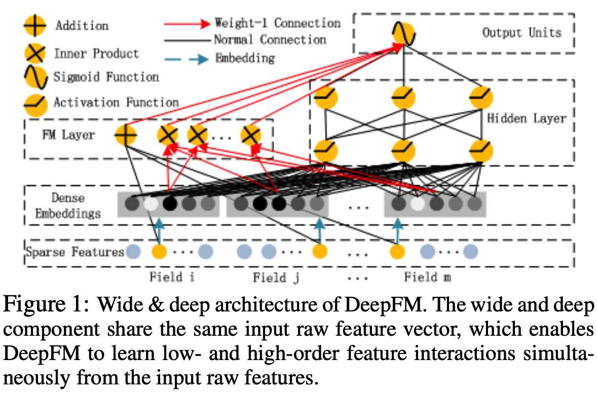
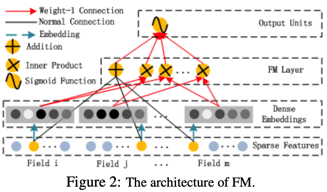
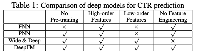
DeepFM(Factorization-Machine based neural network)은 같은 input을 공유하는 FM component(low-order feature interaction 학습) 부분과 Deep component(high-order feature interaction 학습) 부분으로 구성되어있다.(Figure 1)

$\hat{y} = sigmoid(y_{FM} + y_{DNN} ),$ (1)

where $\hat{y} ∈ (0, 1)$ is the predicted CTR, yFM is the output of FM component, and yDNN is the output of deep component.

FM Component

FM(Feature machine) 모델은 (order-1) interaction 뿐 아니라 각 feature latent vectors의 inner product로 pairwise (order-2) interactions을 학습한다.

[특징]: weight 대신 V_i, V_j(latent vectors) 사용함

As Figure 2 shows, the output of FM is the summation of an Addition unit and a number of Inner Product units:

$y_{FM} = <w, x> + \Sigma^d_{j_1=1} \Sigma^d_{j_2=j_1+1} <V_i, V_j> x_{j_1}· x_{j_2},$ (2)

where $w ∈ R^d$ and $V_i ∈ R^k (k\ is\ given)^2$.

The Addition unit (<w, x>) reflects the importance of order-1 features, and the Inner Product units represent the impact of order-2 feature interactions.

• [참고] 참고 youtube 동영상에서 FFM(Field-aware Factorization Machine)으로 설명함
  • 어떠한 Field와 interaction 하는지에 따라 Weight을 다르게 사용하여 학습한다.
  • wide & deep과 다른점: linear로 하던 작업(cross product Transformation) → FM component 부분으로 변경함

Deep Component

Deep Component는 high-order feature interactions를 학습하기 위한 feed-forward neural network이다.

Figure 4 highlights the sub-network structure from the input layer to the embedding layer.

FM model을 통해 latent feature vectors를 학습하기 때문에 pre-training이 필요없어 end-to-end 학습이 가능하다.

Denote the output of the embedding layer as:

$a^{(0)} = [e_1, e_2, ..., e_m],$ (3)

where ei is the embedding of i-th field and m is the number of fields.

Then, a(0) is fed into the deep neural network, and the forward process is:

$a^{(l+1)} = σ(W^{(l)}a^{(l)} + b^{(l)}),$ (4)

where l is the layer depth and σ is an activation function. a(l), W(l), b(l)are the output, model weight, and bias of the l-th layer. (단순 FFN 식과 같음)

최종적으로 sigmoid function을 통과한 CTR prediction:

$y_{DNN} = σ(W^{(|H|+1)}· a^{(H)} + b^{(|H|+1)})$,

where |H| is the number of hidden layers. (논문에 누락?된 괄호 추가함)

We would like to point out the two interesting features of this network structure:

1. while the lengths of different input field vectors can be different, their embeddings are of the same size (k);
   • 보통 embedding layer의 특징임
2. the latent feature vectors (V) in FM now server as network weights which are learned and used to compress the input field vectors to the embedding vectors.
   • FM 먼저 훈련하는 것은 아니고 동시에 훈련(같이 사용한다)

2.2 Relationship with the other Neural Networks

1. FNN(Factorization-machine supported Neural Network)
2. PNN(Product-based Neural Network)
3. Wide & Deep Model

• [예시 참고] wide & deep model from Google
  • Deep에서 훈련: 참새, 비둘기는 날 수 있어 -> 날개 달린 짐승은 날 수 있어
  • Wide에서 훈련 : 펭귄 못 날아
  • Source: https://ai.googleblog.com/2016/06/wide-deep-learning-better-together-with.html

The human brain is a sophisticated learning machine, forming rules by memorizing everyday events (“sparrows can fly” and “pigeons can fly”) and generalizing those learnings to apply to things we haven't seen before (“animals with wings can fly”). Perhaps more powerfully, memorization also allows us to further refine our generalized rules with exceptions (“penguins can't fly”).

Summarizations

: 네 가지 측면에서 다른 딥 모델과 비교해봤을 때, DeepFM은 pre-training과 feature engineering이 필요하지 않은 유일한 모델이며, low- and high-order feature interactions를 모두 capture한다.(Table 1)

[나머지 논문 참고]