반응형

** 아래의 내용은 위의 논문에서 사용되는 사진과 제가 재해석한 내용입니다.
** 첨언 및 조언 환영합니다!


Abstract

우리의 접근법은 hand-desinged componets의 필요성을 효율적으로 제거하여 detection pipeline을 유연하게 한다.

Our approach streamlines the detection pipeline, effectively removing the need for many hand-designed components like a non-maximum suppression procedure or anchor generation that explicitly encode our prior knowledge about the task.


새로운 framework(Detection Tranformer, DETR)의 주요 구성요소는 bipartite matching을 통해 unique한 예측을 강제?하는 set(집합) 기반 global loss와 transformer encoder-decoder architecture이다.

The main ingredients of the new framework, called DEtection TRansformer or DETR, are a set-based global loss that forces unique predictions via bipartite matching, and a transformer encoder-decoder architecture.


학습된 object queries의 fixed small set이 주어지면, DETR은 objects와 glabal image context의 관계에 대해 추론하여 최종 예측 set을 병렬로 출력한다.

Given a fixed small set of learned object queries, DETR reasons about the relations of the objects and the global image context to directly output the final set of predictions in parallel.


1. Introduction

object detection의 목적은 관심있는 각 object의 bounding boxes와 category labels의 set을 예측하는 것이다.

The goal of object detection is to predict a set of bounding boxes and category labels for each object of interest.


우리는 surrogate(대리?,대체?) tasks로 우회하기위한 direct set prediction 접근방법을 목표로 한다.

we propose a direct set prediction approach to bypass the surrogate tasks.


end-to-end philosopht(철학?,연구?)은 machine translation or speech recognition과 같은 complex structured 예측 테스크에서 상당한 발전을 가져왔지만 아직 object detection에서는 아니다.

This end-to-end philosophy has led to significant advances in complex structured prediction tasks such as machine translation or speech recognition, but not yet in object detection: previous attempts [43,16,4,39] either add other forms of prior knowledge, or have not proven to be competitive with strong baselines on challenging benchmarks.

Fig1. DETR

DETER은 모든 objects를 한번에 예측하고 예측된 object와 실제 object간의 bipartite matching을 수행하는 set loss function으로 end-to-end 훈련한다.

Our DEtection TRansformer (DETR, see Figure 1) predicts all objects at once, and is trained end-to-end with a set loss function which performs bipartite matching between predicted and ground-truth objects.

기존 detection 방법과 달리 DETR은 customized layer가 필요하지 않으므로 standard CNN과 transformer classes가 포함된 framework에서 쉽게 재현할 수 있다.

Unlike most existing detection methods, DETR doesn’t require any customized layers, and thus can be reproduced easily in any framework that contains standard CNN and transformer classes.1.


matching loss function은 예측을 gound truth object에 고유하게 할당하고 예측된 objects의 permutation(순열?, 가능한 변수 중 하나)이 변하지 않기 때문에 병렬로 내보낼 수 있다.

Our matching loss function uniquely assigns a prediction to a ground truth object, and is invariant to a permutation of predicted objects, so we can emit them in parallel.


보다 정확하게 DETR은 큰 objects에서 훨씬 더 나은 성능을 보여주며, 결과는 transformer의 on-local computations(로컬 컴퓨터로 계산?)에 의해 가능하다. (의역)

More precisely, DETR demonstrates ignificantly better performance on large objects, a result likely enabled by the on-local computations of the transformer.

하지만, small objects에 관하여 더 낮은 성능을 갖는다.

It obtains, however, lower performances on small objects.


실험에서, 사전 훈련된 DETR 위의 simple segmentation head가 Panoptic Segmentation의 competitive baselines을 능가한다는 것을 보여준다. (4.2확인)

In our experiments, we show that a simple segmentation head trained on top of a pretrained DETR outperfoms competitive baselines on Panoptic Segmentation [19], a challenging pixel-level recognition task that has recently gained popularity.


2. Related work

(논문 참고)


3. The DETR model

Fig 2. DETR model

detection에서 direct set precditions를 위해서는 2가지 필수적인 요소가 있다.

(1) 예측된 box와 실제 box 사이에 고유한 matching을 강제하는 set prediction loss.

(2) object set를 예측하고 그 관계를 모델링하는 architecture.

Two ingredients are essential for direct set predictions in detection:

(1) a set prediction loss that forces unique matching between predicted and ground truth boxes;

(2) an architecture that predicts (in a single pass) a set of objects and models their relation. We describe our architecture in detail in Figure 2.


3.1 Object detection set prediction loss

(이해 잘 안됨, 다시 리뷰하기)


Each element i of the ground truth set can be seen as a yi = (ci , bi) where ci is the target class label (which may be ∅) and bi ∈ [0, 1]^4 is a vector that defines ground truth box center coordinates and its height and width relative to the image size.


Bounding box loss.

The second part of the matching cost and the Hungarian loss is Lbox(·) that scores the bounding boxes. Unlike many detectors that do box predictions as a ∆ w.r.t. some initial guesses, we make box predictions directly.


3.2 DETR architecture

전반적인 DETR architecture는 놀라울 정도로 간단하고 Figure 2에 묘사되어있다.

The overall DETR architecture is surprisingly simple and depicted in Figure 2.


3가지 주요 구성요소가 있다.

  1. compact한 feature representation을 추출하기 위한 CNN backbone
  2. encoder-decoder transformer
  3. 최종 detection 예측을 만드는 간단한 FFN

It contains three main components, which we describe below: a CNN backbone to extract a compact feature representation, an encoder-decoder transformer, and a simple feed forward network (FFN) that makes the final detection prediction.


Inference code for DETR can be implemented in less than 50 lines in PyTorch [32]. (A.6 PyTorch inference cod)

import torch
from torch import nn
from torchvision.models import resnet50

class DETR(nn.Module):
    def __init__(self, num_classes, hidden_dim, nheads,
                             num_encoder_layers, num_decoder_layers):
        super().__init__()
        # We take only convolutional layers from ResNet-50 model
        self.backbone = nn.Sequential(*list(resnet50(pretrained=True).children())[:-2])
        self.conv = nn.Conv2d(2048, hidden_dim, 1)
        self.transformer = nn.Transformer(hidden_dim, nheads,
                                                                          num_encoder_layers, num_decoder_layers)
        self.linear_class = nn.Linear(hidden_dim, num_classes + 1)
        self.linear_bbox = nn.Linear(hidden_dim, 4)
        self.query_pos = nn.Parameter(torch.rand(100, hidden_dim))
        self.row_embed = nn.Parameter(torch.rand(50, hidden_dim // 2))
        self.col_embed = nn.Parameter(torch.rand(50, hidden_dim // 2))

    def forward(self, inputs):
        x = self.backbone(inputs)
        h = self.conv(x)
        H, W = h.shape[-2:]
#         print(self.col_embed[:W].unsqueeze(0).shape, self.row_embed[:H].unsqueeze(1).shape)  # torch.Size([1, 38, 128]) torch.Size([25, 1, 128])
        pos = torch.cat([
            self.col_embed[:W].unsqueeze(0).repeat(H, 1, 1),
            self.row_embed[:H].unsqueeze(1).repeat(1, W, 1),
        ], dim=-1).flatten(0, 1).unsqueeze(1)
        h = self.transformer(pos + h.flatten(2).permute(2, 0, 1),
                                                 self.query_pos.unsqueeze(1))
        return self.linear_class(h), self.linear_bbox(h).sigmoid()

detr = DETR(num_classes=91, hidden_dim=256, nheads=8, num_encoder_layers=6, num_decoder_layers=6)
detr.eval()
inputs = torch.randn(1, 3, 800, 1200)
logits, bboxes = detr(inputs)


Backbone.

ResNet50

Typical values we use are C = 2048 and H, W = $\frac{H_0}{32}, \frac{W_0}{32}$.


Transformer encoder.

First, a 1x1 convolution reduces the channel dimension of the high-level activation map f from C to a smaller dimension d. creating a new feature map z0 ∈ R d×H×W .

The encoder expects a sequence as input, hence we collapse the spatial dimensions of z0 into one dimension, resulting in a d×HW feature map.

Each encoder layer has a standard architecture and consists of a multi-head self-attention module and a feed forward network (FFN).

Since the transformer architecture is permutation-invariant, we supplement it with fixed positional encodings [31,3] that are added to the input of each attention layer.


Transformer decoder.

The decoder follows the standard architecture of the transformer, transforming N embeddings of size d using multi-headed self- and encoder-decoder attention mechanisms.

The difference with the original transformer is that our model decodes the N objects in parallel at each decoder layer, while Vaswani et al.

These input embeddings are learnt positional encodings that we refer to as object queries, and similarly to the encoder, we add them to the input of each attention layer.


Prediction feed-forward networks (FFNs).

The final prediction is computed by a 3-layer perceptron with ReLU activation function and hidden dimension d, and a linear projection layer.

The FFN predicts the normalized center coordinates, height and width of the box w.r.t. the input image, and the linear layer predicts the class label using a softmax function.

Since we predict a fixed-size set of N bounding boxes, where N is usually much larger than the actual number of objects of interest in an image, an additional special class label ∅ is used to represent that no object is detected within a slot. (“background” class와 비슷한 역할을 함)


Auxiliary decoding losses.

We add prediction FFNs and Hungarian loss after each decoder layer. All predictions FFNs share their parameters.


4. Experiments

자세한 사항 (논문참고)

Technical details values
optimizer AdamW
transformers' learning rate $10^{-4}$
backborne's lr $10^{-5}$
weight decay $10^{-4}$
backbones ResNet50, ResNet-101

4.4 DETR for panoptic segmentation

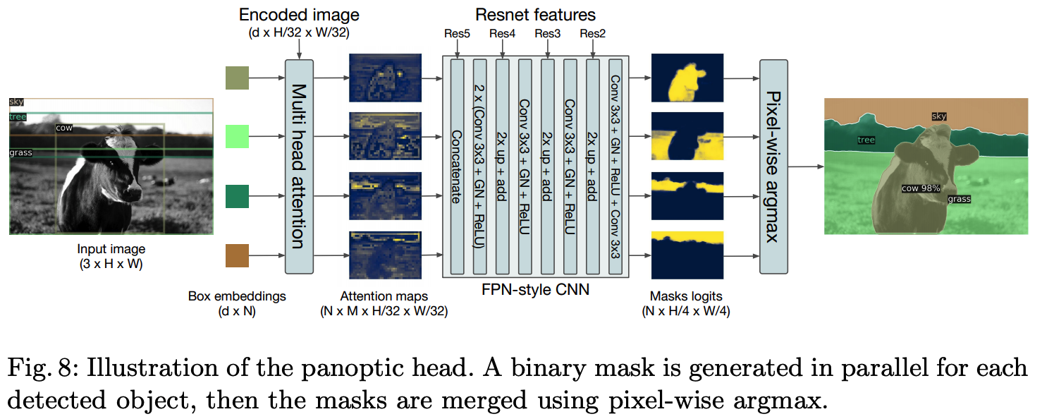
Panoptic segmentation [19] has recently attracted a lot of attention from the computer vision community. Similarly to the extension of Faster R-CNN [37] to Mask R-CNN [14], DETR can be naturally extended by adding a mask head on top of the decoder outputs.

Fig 8. DETR Segmentation

Predicting boxes is required for the training to be possible, since the Hungarian matching is computed using distances between boxes.

We also add a mask head which predicts a binary mask for each of the predicted boxes, see Figure 8.

It takes as input the output of transformer decoder for each object and computes multi-head (with M heads) attention scores of this embedding over the output of the encoder, generating M attention heatmaps per object in a small resolution.


5. Conclusion

direct set prediction을 위한 transformers와 bipartite matching loss를 기반으로 object detection system을 위한 새로운 구조인 DETR을 소개했다.

We presented DETR, a new design for object detection systems based on transformers and bipartite matching loss for direct set prediction.

self-attention을 이용한 global information processing 덕분에 Faster R-CNN보다 large objects에 대해 훨씬 더 나은 성능을 달성한다.

In addition, it achieves significantly better performance on large objects than Faster R-CNN, likely thanks to the processing of global information performed by the self-attention.


나의 결론

장점 :

  1. Transformer를 Vision task에서 적용함
  2. 기존에 사용하던 ResNet과 Transformer를 이용하여 간단한 basic 코드로 large object의 detection 성능을 높임
  3. pre-trained DETR 위에 간단한 Multi-head attention을 활용하여 segmentation task에 사용할 수 있음

단점(아쉬운 점) :

small object, 겹치는 object의 detection 성능 향상이 필요할 것으로 보임

반응형
반응형

[논문]

A Style-Based Generator Architectur for Generative Adversarial Networks


[코드]

NVlabs/stylegan


** 아래의 내용은 위의 논문에서 사용되는 사진과 제가 재해석한 내용입니다.
** 첨언 및 조언 환영합니다!


Abstract

new architecture는 generated(생성된) images에서 높은 수준의 attributes와 stochastic variation을 자동으로 학습하고, 이는 synthesis에 대한 직관적이고 scale-specific control을 가능하게 한다.

The new architecture leads to an automatically learned, unsupervised separation of high-level attributes and stochastic variation in the generated images, and it enables intuitive, scale-specific control of the synthesis.


interpolation 품질과 disentanglement를 정량화하기위해 모든 generator architecture에 적용할 수 있는 두 가지 새로운 자동화 방법을 제안한다.

To quantify interpolation quality and disentanglement, we propose two new, automated methods that are applicable to any generator architecture.

  • interpolation

    : In the mathematical field of numerical analysis, interpolation is a type of estimation, a method of constructing new data points within the range of a discrete set of known data points.

    출처: https://en.wikipedia.org/wiki/Interpolation

  • Disentanglement

    : as typically employed in literature, refers to independence among features in a representation.

    출처: https://arxiv.org/pdf/1812.02833


1. Introduction

generators는 계속해서 black boxes로 작동하고 있으며 최근 노력에도 불구하고 image synthesis process의 다양한 측면에서의 이해가 여전히 부족하다.

Yet the generators continue to operate as black boxes, and despite recent efforts, the understanding of various aspects of the image synthesis process, e.g., the origin of stochastic features, is still lacking.


Our generator는 학습된 constant input에서 시작하여 latent code 기반으로 각 convolution layer에서 이미지의 "style"을 조정하므로 다양한 scales에서 이미지 feature의 strength를 직접적 제어한다.

Our generator starts from a learned constant input and adjusts the “style” of the image at each convolution layer based on the latent code, therefore directly controlling the strength of image features at different scales.


우리는 discriminator나 loss function을 수정하지 않는다.

We do not modify the discriminator or the loss function in any way, and our work is thus orthogonal to the ongoing discussion about GAN loss functions, regularization, and hyper-parameters.


두 가지 새로운 자동화 metrics(perceptural path length와 linear separability)를 제안한다.

As previous methods for estimating the degree of latent space disentanglement are not directly applicable in our case, we propose two new automated metrics —perceptual path length and linear separability — for quantifying these aspects of the generator. Using these metrics, our generator admits a more linear, less entangled representation of different factors of variation.


Finally, we present a new dataset of human faces (Flickr-Faces-HQ, FFHQ).


2. Style-based generator

Style GAN Figure 1.

Given a latent code z in the input latent space Z, a non-linear mapping network f : Z → W first produces w ∈ W (Figure 1b, left).

  • y = (Figure 1b A)

For simplicity, we set the dimensionality of both spaces to 512, and the mapping f is implemented using an 8-layer MLP, a decision we will analyze in Section 4.1. Learned affine transformations then specialize w to styles y = (ys, yb) that control adaptive instance normalization (AdaIN) [27, 17, 21, 16] operations after each convolution layer of the synthesis network g.

  • IN (Instance Normalization)

    $IN(x) = \gamma (\frac{x - \mu(x)}{\sigma(x)}) + \beta$

  • AdaIN ( Adaptive Instance Normalization)

    $AdaIN(x_i, y) = y_{s,i} \frac{x_i - \mu}{\sigma(s_i)} + y_{b,i}$ (Eq.1)

where each feature map xi is normalized separately, and then scaled and biased using the corresponding scalar components from style y. Thus the dimensionality of y is twice the number of feature maps on that layer.


AdaIN은 효율성과 간결한 representation으로 우리의 목적에 특히 적합하다.

AdaIN is particularly well suited for our purposes due to its efficiency and compact representation.


explicit(명시적?) noise inputs을 도입하여 stochastic detail을 생성할 수 있는 직접적인 방법을 generator에 제공한다.

Finally, we provide our generator with a direct means to genertate stochastic detail by introducing explicit noise inputs.


2.1. Quality of generated images

Style GAN Table 1.

마지막으로 결과를 더욱 향상시키는 noise inputs과 neighboring styles을 decorrelates(역상관?/비상관?)하고 생성된 이미지를 보다 fine-grained colntrol 할 수 있는 mixing regularizations를 소개한다.

Finally, we introduce the noise inputs (E) that improve the results further, as well as novel mixing regularization (F) that decorrelates neighboring styles and enable more fine-grained control over the generated imagery (Section 3.1)

  • Section 3.1 참고, mixing reluarization은 network가 인접한 style이 correlated 관계가 있다고 가정하는 것을 방지하는 기술이다.

    3.1. Style mixing | This regularization(mixing regularization) technique prevents the network from assuming that adjacent styles are correlated.


2.2. Prior art

[details 논문 참조]


3. Properties of the style-based generator

genertor architecture를 사용하면 scale-specific 수정을 통해 이미지 합성(synthesis)을 컨트롤할 수 있다.

Our generator architecture makes it possible to control the image synthesis via scale-specific modifications to the styles.


각 style은 next AdaIN operation에 overridden(재정의)되기 전에 하나의 convolution만 제어한다.

Thus each style controls only one convolution before being overridden by the next AdaIN operation.


[details 논문 참조]


4. Disentanglement studies

[논문 참조]


5. Conclusion

high-level attribute와 stochastic effects의 분리와 intermediate latent space에 대한 연구가 GAN synthesis의 이해와 controllability의 개선에 유익한 것으로 입증되었다고 믿는다.

This is true in terms of established quality metrics, and we further believe that our investigations to the separation of high-level attributes and stochastic effects, as well as the linearity of the intermediate latent space will prove fruitful in improving the understanding and controllability of GAN synthesis.


나의 결론

  • 장점: controllable generator 아이디어 연구 및 입증, FFHQ dataset 제공
  • 단점: generator 부분에 포커싱됨, Discriminator에 대한 논의가 없는 것 아쉬움


StyleGAN2

[StyleGAN2 논문]

[NVlabs/stylegan2 코드]

반응형
반응형

Tensorflow serving 하기

TensorFlow Serving을 사용하면 동일한 서버 아키텍처와 API를 유지하면서 새로운 알고리즘과 실험을 쉽게 배포 할 수 있습니다. TensorFlow Serving은 TensorFlow 모델과의 즉각적인 통합을 제공하지만 다른 유형의 모델 및 데이터를 제공하도록 쉽게 확장 할 수 있습니다.(출처: tensorflow.org)


참조

Train and serve a TensorFlow model with TensorFlow Serving | TFX

TensorFlow Serving with Docker | TFX

모델 저장

# >> 추후 모델 업데이트를 위해 version별로 모델 저장함
## tensorflow version 2.3.1
model_path='models'
model_name='my_model'
model.save(f'{model_path}/{model_name}/1')

저장된 모델 확인

## model format check
for root, dirs, files in os.walk(os.path.join(model_path, model_name)):
    indent = '    ' * root.count(os.sep)
    print('{}{}/'.format(indent, os.path.basename(root)))
    for filename in files:
        print('{}{}'.format(indent + '    ', filename))

## output format ex)
# 1/
#             .DS_Store
#             saved_model.pb
#             variables/
#                 variables.data-00000-of-00001
#                 variables.index
#             assets/
## ex
$ export model_path='models'
$ export model_name='my_model'

## model input, output shape check
$ saved_model_cli show --dir ${model_path}/${model_name}/1 --tag_set serve \
                       --signature_def serving_default

Serving with Docker

TensorFlow Serving을 시작하는 가장 쉬운 방법 중 하나는 Docker를 사용하는 것 입니다. (출처: tensorflow.org)

Docker 설치하기

(on MacOS)

큐베플로우 설치 on MacOS

(others)

https://www.tensorflow.org/tfx/serving/docker#install_docker

## !!도커 설치가 선행되어야함!! ##

## tensorflow에서 제공하는 이미지 가장 최신버전으로 다운로드(현재 기준 2.3.0)
$ docker pull tensorflow/serving
# image 생성 체크
$ docker image ls
# image 삭제
$ docker image rm <IMAGE ID>
# ex
$ export container_name='serving_base'

## tensorflow/serving container 띄우기
$ docker run -d --name ${container_name} -it --rm \
        -p 8500:8500 \
        -p 8501:8501 \
        -v "$(pwd)/${model_path}/${model_name}:/${model_path}/${model_name}" \
        -e MODEL_NAME=${model_name} \
                tensorflow/serving &

# container 생성 체크
$ docker container ls

# container 삭제
# issue: Bind for x.x.x.x:port# failed: port is already allocated.
$ docker rm -f <NAMES>

docker container ls

모델 실행 (REST API)

rest api port: 8501

import json
import numpy
import requests
data = json.dumps({"signature_name": "serving_default",
                   "instances": x.numpy().tolist()})  # json dumps를 위해 list로 변경 (shape 확인 필수)
headers = {"content-type": "application/json"}
json_response = requests.post(f'http://localhost:8501/v1/{model_path}/{model_name}:predict',
                              data=data, headers=headers)
predictions = numpy.array(json.loads(json_response.text)["predictions"])
print(predictions)
반응형
반응형

EfficientNet: Rethinking Model Scaling for Convolutional Neural Networks

[Efficient Net 논문]

arxiv.org/pdf/1905.11946.pdf


** 아래의 내용은 위의 논문에서 사용되는 사진과 제가 재해석한 내용입니다.


[코드]

github.com/tensorflow/tpu/tree/master/models/official/efficientnet


예시)

Top 4 Pre-Trained Models for Image Classification with Python Code


Abstract

관찰을 바탕으로, 단순하지만 매우 효과적인 compound coefficient를 사용하여 depth(깊이)/width(너비)/resolution(해상도)의 모든 dimension을 균일하게 scale..하는 새로운 scaling 방법을 제안한다.

Based on this observation, we propose a new scaling method that uniformly scales all dimensions of depth/width/resolution using a simple yet highly effective compound coefficient.


MobileNets과 ResNet을 scaling up 할 때 이 방법의 효과를 볼 수 있다.

We demonstrate the effectiveness of this method on scaling up MobileNets and ResNet.


1. Introduction

ConvNets(Convolution Networks)를 scaling up(확장)하는 과정을 연구하고 재고하고자 한다.

In this paper, we want to study and rethink the process of scaling up ConvNets.


우리(Google Research, Brain Team)의 경험적 연구에 따르면 network width/depth/resolution의 모든 dimensions의 균형을 맞추는 것이 중요하며, 놀랍게도 이러한 균형은 단순히 일정한 비율로 각 크기를 조절하여 달성할 수 있다.

Our empirical study shows that it is critical to balance all dimensions of network width/depth/resolution, and surprisingly such balance can be achieved by simply scaling each of them with constant ratio.


그러나 우리가 아는 한 우리는 network width/depth/resolution의 모든 dimensions간의 관계를 경험적(?)으로 정량화한 최초의 기업이다.

but to our best knowledge, we are the first to empirically quantify the relationship among all three dimensions of network width, depth, and resolution.


efficientnet_fig1

Figure 1은 EfficientNets이 다른 ConvNets을 훨씬 능가하는 ImageNet 성능을 요약한 것이다.

Figure 1 summarizes the ImageNet performance, where our EfficientNets significantly outperform other ConvNets.


2. Related Work

ConvNet Accuracy:

많은 application에서 더 높은 정확도가 중요하지만 이미 HW 메모리 한계에 도달했기때문에 더 높은 accuracy를 얻으려면 더 나은 efficiency이 필요하다.

Although higher accuracy is critical for many applications, we have already hit the hardware memory limit, and thus further accuracy gain needs better efficiency.

ConvNet Efficiency:

이 논문에서는 state-of-the-art accuracy를 능가하는 super large ConvNets model efficiency를 연구하는 것이 목표다. 이 목표를 달성하기 위해 모델 scaling을 이용한다.

In this paper, we aim to study model efficiency for super large ConvNets that surpass state-of-the-art accuracy. To achieve this goal, we resort to model scaling.

Model Scaling:

network width, depth, and resolutions의 3가지 dimensions 모두에 대해 ConvNet scaling을 체계적이고 경험적으로 연구한다.

Our work systematically and empirically studies ConvNet scaling for all three dimensions of network width, depth, and resolutions.

3. Compound Model Scaling

3.1. Problem Formulation

ConvNet layers는 (모든 Conv가 그런 것은 아니지만) 여러 단계로 분할되며 각 단계의 모든 layers는 동일한 architecture를 공유한다.

(의역)

ConvNet layers are often partitioned into multiple stages and all layers in each stage share the same architecture: ex) ResNet

Therefore, we can define a ConvNet as:

efficientnet_1
efficientnet_fig2


$\hat{F_{1}}$ : layer architecture/baseline network

$\hat{L_{1}} , \hat{W_{1}}$ : the network length, width

$\hat{H_{1}} , \hat{C_{1}}$ : resolution


보통 ConvNet designs에서 가장 좋은 architecture를 찾는 것에 집중했던 것과 달리, model scaling은 미리 정의한 baseline network 변경 없이 network length, width, and/or resolution을 확장하는 것을 시도한다.

Unlike regular ConvNet designs that mostly focus on finding the best layer architecture $\hat{F_{1}}$, model scaling tries to expand the network length, width, and/or resolution without changing $\hat{F_{1}}$ predefined in the baseline network.


우리의 목표는 주어진 resource의 제약에 따라 모델 정확도를 최대화하는 것이다.

Our target is to maximize the model accuracy for any given resource constraints, which can be formulated as an optimization problem:

efficientnet_2

where **w, d, r are coefficients for scaling network width, depth, and resolution; $\hat{F_{1}}, \hat{L_{1}}, \hat{H_{1}}, \hat{W_{1}}, \hat{C_{1}}$ are predefined parameters in baseline network (see Table 1 as an example)


3.2. Scaling Dimensions

efficientnet_fig4

Depth (d): Scaling network depth is the most common way used by many ConvNets.

The intuition is that deeper ConvNet can capture richer and more complex features, and
generalize well on new tasks. However, deeper networks are also more difficult to train due to the vanishing gradient problem. (Although several techniques, such as skip connections and batch normalization.)

Width (w): Scaling network width is commonly used for small size models.

wider networks tend to be able to capture more fine-grained features and are easier to train. However, extremely wide but shallow networks tend to have difficulties in capturing higher level features.

Resolution (r): With higher resolution input images, ConvNets can potentially capture more fine-grained patterns.

the results of scaling network resolutions, where indeed higher resolutions improve accuracy, but the accuracy gain diminishes for very high resolutions (r = 1.0 denotes resolution 224x224 and r = 2.5 denotes resolution 560x560)


관찰 1 - network width, depth, or resolution의 dimension 중 하나라도 scaling up하면 accuracy가 향상되지만 bigger models에서는 accuracy 향상을 기대하기 어렵다.

(의역)

Observation 1 – Scaling up any dimension of network width, depth, or resolution improves accuracy, but the accuracy gain diminishes for bigger models.


3.3. Compound Scaling

efficientnet_fig4

We empirically observe that different scaling dimensions are not independent.


관찰 2 - 더 나은 accuracy와 efficiency를 위해, ConvNet scaling할 때 network width, depth, and resolution의 모든 dimensions의 밸런스가 중요하다.

Observation 2 – In order to pursue better accuracy and efficiency, it is critical to balance all dimensions of network width, depth, and resolution during ConvNet scaling.

In this paper, we propose a new compound scaling method, which use a compound coefficient φ to uniformly scales network width, depth, and resolution in a principled way:

efficientnet_3

where α, β, γ are constants that can be determined by a small grid search.


4. EfficientNet Architecture

모델 스케일링은 baseline network의 layer operators를 변경하지 않기때문에, 좋은 baseline network를 사용하는 것이 중요하다.

Since model scaling does not change layer operators $\hat{F_{1}}$ in baseline network, having a good baseline network is also critical.


우리의 scaling 방법으로 이미지 존재하는 ConvNets를 이용할 것이지만 우리의 scaling 방법의 effectiveness의 더 나은 증명을 위해, 새로운 mobile-size baseline인 EfficientNet 또한 개발했다.

We will evaluate our scaling method using existing ConvNets, but in order to better demonstrate the effectiveness of our scaling method, we have also developed a new mobile-size baseline, called EfficientNet.

efficientnet_table1

Our search produces an efficient network, which we name EfficientNet-B. Since we use the same search space as (Tan et al., 2019), the architecture is similar to MnasNet, except our EfficientNet-B0 is slightly bigger due to the larger FLOPS target (our FLOPS target is 400M).


** MnasNet: Platform-Aware Neural Architecture Search for Mobile

https://arxiv.org/pdf/1807.11626.pdf


baseline EfficientNet-B0을 시작하며, 우리의 compound scaling method를 scale up하는 2가지 step을 제안한다.

Starting from the baseline EfficientNet-B0, we apply our compound scaling method to scale it up with two steps:

  • STEP 1: we first fix φ = 1, assuming twice more resources available, and do a small grid search of α, β, γ based on Equation 2 and 3. In particular, we find the best values for EfficientNet-B0 are α = 1.2, β = 1.1, γ = 1.15, under constraint of α · β 2· γ 2 ≈ 2.
  • STEP 2: we then fix α, β, γ as constants and scale up baseline network with different φ using Equation 3, to obtain EfficientNet-B1 to B7 (Details in Table 2).

우리의 방법은 작은 규모의 baseline network에서 한번만 search(a small grid search of α, β, γ)를 한 다음(1단계) 한 다음 다른 모든 모델(different compound coefficient φ)에 대해 동일한 scaling coefficients를 사용하여(2단계) 이 문제를 해결한다.

Our method solves this issue by only doing search once on the small baseline network (step 1), and then use the same scaling coefficients for all other models (step 2).


5. Experiments

** 논문 참고

efficientnet_table2


6. Discussion

efficientnet_fig8


일반적으로, 모든 scaling 방법은 accuracy가 향상된다. 하지만 우리의 compound scaling 방법은 다른 single-dimension scaling 방법보다 더욱 더 accuracy가 향상시킬 수 있다.

In general, all scaling methods improve accuracy with the cost of more FLOPS, but our compound scaling method can further improve accuracy, by up to 2.5%, than other single-dimension scaling methods, suggesting the importance of our proposed compound scaling.


efficientnet_fig7

위의 그림을 보면, compound scaling 모델이 더 개체의 details한 relevant regions에 더 focusing하는 경향이 있다.

As shown in the figure, the model with compound scaling tends to focus on more relevant regions with more object details.


7. Conclusion

ConvNet scaling을 체계적으로 연구하고, network width, depth을 주의 깊게 조정하는 것과 중요하지만 놓치고 있던 resolution(해상도)를 주의 깊게 조정하지 않는 것이 정확성과 효율성을 향상을 방해한다는 것을 확인했다.

(의역)

In this paper, we systematically study ConvNet scaling and identify that carefully balancing network width, depth, and resolution is an important but missing piece, preventing us from better accuracy and efficiency.


compound scaling 방법으로 구동(?)되는 mobile-size EfficientNet 모델이 매우 효과적으로 scaled up될 수 있다는 것을 증명한다(?)

Powered by this compound scaling method, we demonstrate that a mobile-size EfficientNet model can be scaled up very effectively, surpassing state-of-the-art accuracy with an order of magnitude fewer parameters and FLOPS, on both ImageNet and five commonly used transfer learning datasets.


나의 결론

  • 장점: compound scaling(width, depth, resolution) 방법을 경험적으로 식을 구현(formulated)할 수 있게 되었다는 점에서 큰 도약(?)임. classification 시 object를 더 잘 인식하여 분류할 수 있을 것으로 기대됨
  • 단점: 확장성에 대한 의문..? compound scaling을 여러 ConvNet에 대한 테스트 해봐야할 듯 (모든 layers가 동일한 architecture를 공유하는 ConvNets에 한정된다)


** 첨언 및 조언 환영합니다!

반응형

+ Recent posts