1. Generative Model 이란

판별모델링 vs 생성모델링

• 판별모델링: sample x가 주어졌을 때 레이블 y의 확률 $p(y|x)$를 추정
• 생성모델링: sample x의 관측확률 $p(x)$를 추정, supervised learning의 경우 확률 $p(x|y)$를 추정

→ Goal: sample로 모델을 훈련 (distribution) → sample에 있을 법한 x 생성하기

generative model은 데이터 범주의 분포를, disciriminative model은 결정경계를 학습한다.

generative model은 사후확률을 간접적으로, disciriminative model은 직접적으로 도출한다.

기존 확률적 생성 모델의 난관

1. 특성 간에 조건부 의존성이 매우 클 때 어떻게 대처할 것인가?
2. 모델이 어떻게 고차원 표본 공간의 생성 가능한 샘플 중 만족할만한 하나를 찾을 것인가?

전통적인 확률생성모델은 하나의 확률분포 표현식 $P(X)$를 정의해야하는데, 일반적으로 다변량 결합확률분포의 밀도함수 $p(X_1,X_2,\cdots, X_N)$이며, 이에 기반해 likelihood 예측을 최대화한다(MLE).

이 과정에서 확률추론 계산이 빠질 수 없는데, 확률모델은 랜덤변수가 많을 때 매우 복잡해지기 때문에 확률 계산도 매우 어려워진다. 근사 계산을 한다고 하더라도 효과는 만족스럽지 못할 때가 많다.

⇒ Representation Learning (deep learning이 잘하는 것)

: 고차원 표본공간을 직접 모델링 하는 것이 아니라 저차원의 잠재공간(latent vector)을 사용해 훈련 셋의 각 샘플을 표현하고 이를 원본 공간의 포인트에 매핑하는 것

= 잠재공간의 각 포인트는 어떤 고차원 이미지에 대한 representation

2. VAE (AE)

AE (Auto-Encoder)

• 인코더: 고차원 입력데이터를 저차원 representation vector로 압축
• 디코더: 주어진 representation vector를 원본 차원으로 다시 압축을 해제

→ AE는 각 이미지가 잠재공간의 한 포인트에 직접 매핑됨

VAE (Variational Auto-Encoder)

VAE는 각 이미지를 잠재 공간에 있는 포인트 주변의 Multivariate Normal distribution에 매핑

• Encoder
  • latent vector ( zero-mean Gaussian )$\sigma = exp(log(var)/2)$
  • $\epsilon \sim N(0,1)$
  • $z = \mu + \sigma * \epsilon$
  • 분산에 log를 취하는 이유: 신경망 유닛의 일반적인 출력은 $(-\infin, \infin)$범위의 모든 실수지만 분산은 항상 양수임
  • 평균과 벡터만 매핑하는 이유: VAE는 latent vector의 차원 사이에는 어떠한 상관관계가 없다고 가정함
• Decoder⇒ 계산이 어렵기 때문에 KLD가 줄어드는 쪽으로 $q(z)$를 근사하는 방법으로 적용한다.
  • KLDivergence : 두 모델 분포들 간 얼마나 가까운지에 대한 정보 손실량의 기대값 (Symmetry하지 않음)
  • $D_{KL}(p||q) = E[log(p_i)-log(q_i)] = \Sigma_i p_i log\frac{p_i}{q_i}$
• $q(z|x)$: 다변량 정규분포로 봄
• encoder가 만든 𝑧를 받아서 원 데이터 𝑥'를 복원: $p(z|x)$

3. GAN

: Generative Model을 훈련시키는 방법 idea

1. generator(생성알고리즘): 생성한 데이터를 discriminator가 진짜로 인식하도록 하는 것이 목표
2. discriminator(판별알고리즘): generator로 부터 전달된 데이터를 가짜로 인식하도록 하는 것이 목표

→ 두 가지 네트워크가 서로 적대적(Adversarial)인 관계임

• train 구조

• minimax objective function학습의 의미: V(D,G)가 최대가 되도록 학습하는 것은 판별자(D), 최소화되도록 학습하는 것은 생성자(G)

• issue
  1. 진동하는 loss (= 불안정)
  2. 유용하지 않은 loss (훈련방법이 기존과 달라서 이해하기 어려운 loss)
  3. mode collapse
  4. : 생성자가 판별자를 속일 수 있는 하나의 샘플(=mode)을 찾아내려는 경향이 있음
  5. hyper parameter (많고, 민감함) → 훈련이 어려움

4. Vision GAN

: GAN을 여러 데이터에 훈련시키는 방법 idea (based Vision Task)

Basic) convonvolution

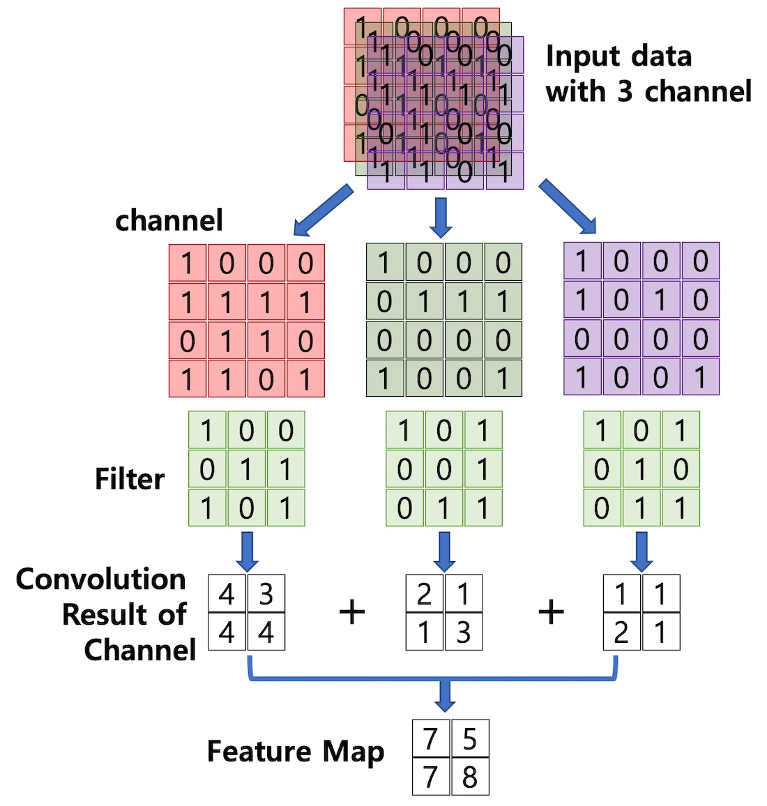
• Convolition: 필터를 이미지의 일부분과 픽셀끼리 곱한 후 결과를 더하는 것
  • filter: 컬러 이미지의 경우 3개의 채널을 가짐, 여러개의 필터를 가짐
  • (이미지의 영역과 필터가 비슷할수록 큰 양수가 출력되고 반대일수록 큰 음수가 출력됨)
  • stride: 필터가 한 번에 입력 위를 이동하는 크기 → 채널의 수는 늘리고 텐서의 공간 방향 크기를 줄이는 데 사용할 수 있음
  • padding: padding="same"의 경우 입력 데이터를 0으로 패딩하여 strides=1일 때 출력의 크기를 입력 크기와 동일하게 만듬
• 필터를 전체 이미지에 대해 왼쪽에서 오른쪽으로 위에서 아래로 이동하면서 합성곱의 출력을 기록

DCGAN

"GANs이 합성곱을 만났을 때!"

CNN은 이미지를 분할하여 화소 위치와 관련된 정보를 대량으로 유실한다. 분류 문제는 잘 해결할 수 있지만 고해상도를 가진 이미지를 출력할 수 없다.

→ Fractional-Strided Convolutions (deconvolutions)

각 층의 높이와 넓이가 줄지 않고 오히려 커져 최종적인 출력과 원래 입력이미지의 크기가 동일할 수 있도록 만들어줌

• Conv_Transpose2D (=deconvolutions)

1. 파란 부분: original 이미지
2. 이미지 사이에 padding 추가
3. filter 통과

• $Output\ Size = (input\ size -1)* stride + 2*padding + (kernel\ size)$

• Architecture guidelines for stable Deep Convolutional GANs
  • Fully connected layer와 Pooling layer를 최대한 배제하고 Strided Convolution과 Transposed Convolution으로 네트워크 구조를 만들었습니다. Fully connected layer와 Max-pooling layer는 매개변수의 수를 줄일 수 있지만 이미지의 위치 정보를 잃어 버릴 수 있다는 단점이 있습니다.
  • Generator와 Discriminator에 배치 정규화(Batch Nomalization)을 사용하였습니다. 이는 입력 데이터가 치우쳐져 있을 경우의 평균과 분산을 조정해주는 역할을 합니다. 따라서 back propagation을 시행했을 때 각 레이에어 제대로 전달되도록해 학습이 안정적으로 이루어지는데 중요한 역할을 하였습니다.
  • 마지막 layer를 제외하고 생성자의 모든 layer에 ReLU activation를 사용하였습니다. 마지막 layer에는 Tanh를 사용하였습니다.
  • Discriminator의 모든 레이어에 LeakyReLU를 사용하였습니다.
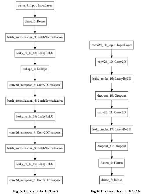
  • Architecture summary

[test image]

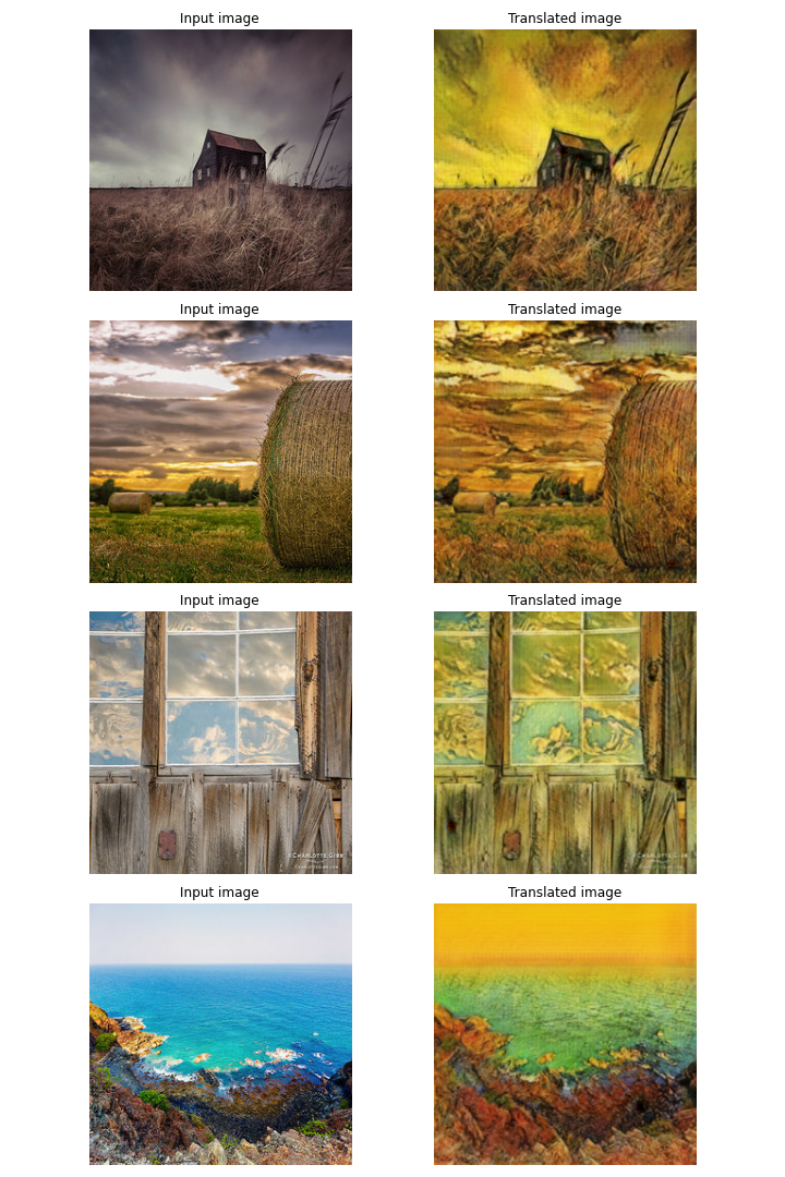
CycleGAN

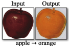
목적: 도메인 A의 이미지를 도메인 B의 이미지로 혹은 그 반대로 바꾸는 모델 훈련하기

• 유효성, 재구성, 동일성의 3박이 잘 이루어져야 훈련이 잘 됨
  1. 유효성 : 도메인 A의 이미지를 도메인 B의 이미지로 혹은 그 반대로 바꾸기 (기존 GAN loss) → $G_{BA}(b)=fake_a\ or\ G_{AB}(a) = fake_b$
  2. 재구성(cycle consistency loss) : 도메인 A의 이미지를 도메인 B의 이미지로 또 다시 도메인 A의 이미지로 바꾸기(원래 도메인에 해당하는 이미지로 돌아오는 가?) → $G_{AB}(G_{BA}(b))=reconstr_b \ or \ G_{BA}(G_{AB}(a))=reconstr_a$→ $X$와 $\hat{X}$사이에서 평균 절대 오차 계산
  3. 동일성(Identity loss) : ( 도메인 A에서 도메인 B으로 Generate하는 모델에 도메인 B 이미지를 넣었을 때 다시 B 도메인의 이미지로 생성을 할 수 있는가? ) $G_{BA}(a)= a \ or\ G_{AB}(b)= b$$Identity\ loss = |G(Y)-Y| + |F(X)-X|$ ⇒ 이미지에서 변환에 필요한 부분 이외에는 바꾸지 않도록 생성자에 제한을 가함

** cycleGAN과 pix2pix의 주된 차이점: 추가 손실 함수(cycle consistency loss)를 사용하여 쌍으로 연결된 데이터없이도 훈련을 할 수 있다. (pair 데이터를 구하기 어려움)

[test image]

5. NLP Generate Model

• 이미지와 텍스트 데이터가 다른 점
  1. 텍스트 데이터는 개별적인 데이터 조각(문자나 단어)로 구성, 반면 이미지의 픽셀은 연속적인 색상스펙트럼 위의 한 점
  2. 텍스트 데이터는 시간 차원이 있지만 공간 차원은 없음, 이미지 데이터는 두 개의 공간 차원이 있고 시간 차원은 없음
  3. 텍스트 데이터는 개별 단위의 작은 변화에도 민감
  4. 텍스트 데이터는 규칙 기반을 가진 문법 구조
• paper) MODERN METHODS OF TEXT GENERATION (2020)
  • https://arxiv.org/pdf/2009.04968.pdf

Basic

1. RNN: 시퀀스의 다음 단어 하나를 예측하는 것이 목적
   1. 기존 단어의 시퀀스를 네트워크에 주입하고 다음 단어를 예측
   2. 이 단어를 기존 시퀀스에 추가하고 과정을 반복
2. Encoder-Decoder (ex, Seq2seq): 입력 시퀀스에 관련된 완전히 다른 단어의 시퀀스를 예측
   1. 원본 입력 시퀀스는 인코더의 RNN에 의해 하나의 벡터로 요약 → 문맥 벡터(context vector) : 이 벡터는 디코더 RNN의 초깃값으로 사용
   2. 각 타임스텝에서 디코더 RNN의 은닉 상태는 완전 연결 층에 연결되어 단어 어휘 사전에 대한 확률 분포를 출력(-) 긴 문장의 시작 부분에 정보는 문맥 벡터에 도달할 때 희석될 수 있음
   3. 언어번역, 질문-대답 생성, 텍스트 요약
3. Attention: 인코더의 이전 은닉 상태와 디코더의 현재 은닉 상태를 문맥 벡터 생성을 위한 덧셈 가중치로 변환하는 일련의 층

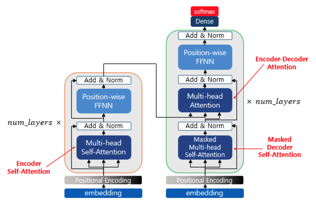
Transformer (Attention Is All You Need)

AutoEncoder-Decoder 구조 (Seq2Seq 유사)

(개인적인 생각) GAN과 유사한 방법은 Electra or GPT

Elactra paper: https://arxiv.org/pdf/2003.10555.pdf

GPT paper: https://s3-us-west-2.amazonaws.com/openai-assets/research-covers/language-unsupervised/language_understanding_paper.pdf

6. Multi-modal GAN

Zero-Shot Text-to-Image Generation [DALL*E]

• paper) zero-shot text-to-image generation (2021)
  • https://arxiv.org/pdf/2102.12092.pdf
  • Results : https://openai.com/blog/dall-e
• 참고
  • https://www.youtube.com/watch?v=az-OV47oKvA&t=3s

reference

(book) 미술관에 GAN 딥러닝 실전 프로젝트

• Paper
  • https://arxiv.org/pdf/1301.3781v3.pdf
• References
  • Word2Vec : https://wikidocs.net/22660
  • Natural Language Processing: https://web.stanford.edu/class/cs224n/readings/cs224n-2019-notes01-wordvecs1.pdf
  • Word2Vec 학습 방식: https://ratsgo.github.io/from%20frequency%20to%20semantics/2017/03/30/word2vec/
  • 쉽게 쓰여진 word2vec: https://dreamgonfly.github.io/blog/word2vec-explained/

[사전학습] NLP Basic

: 텍스트 기반의 모델을 만들기 위해서는 우선 사람의 언어인 텍스트를 모델이 이해할 수 있도록 숫자로 바꾸어야 한다.

Tokenizer란

언어적 특성을 반영해 단어를 수치화하기 위해 문장을 명사, 동사, 형용사, 조사 등 의미 단위로 나눈다.

Python으로 딥러닝하기 | 자연어 처리 1. 토크나이징

Word Embedding이란

단어를 벡터로 바꾸는 모델을 Word embedding model이라고 부른다.

Frequency based 과 Prediction based를 각각 다루고자 했으나 아래의 블로그를 참고..

*참고: 빈도수 세기의 놀라운 마법 Word2Vec, Glove, Fasttext

• Sparse Representation

ex) one-hot vector: 표현하고자 하는 단어의 인덱스 값만 1, 나머지 인덱스는 전부 0으로 표현되는 방법 → "localist" representation

한계: 단어와 단어 간의 관계가 전혀 드러나지 않아 벡터에 단어의 의미를 담을 수 없다.

벡터 또는 행렬(matrix)의 값이 대부분이 0으로 표현되는 방법을 희소 표현(sparse representation)이라고 한다.

• Dense(distributed) Representation

분포 가설 가정: **'비슷한 위치(문맥)에서 등장하는 단어들은 비슷한 의미를 가진다'**라는 가정한다.한계: '단어 동시 등장 정보'를 가정하는 방법의 경우 의미상 아무런 관련이 없어 보이는 단어임에도 벡터공간에 매우 가깝게 임베딩되는 사례가 발생하곤 한다.

장점: 단어 벡터가 단어 간 유사도(의미)를 반영한 값을 가진다.

분산 표현(distributed representation) 방법은 단어의 의미를 여러차원에 분산하여 표현하는 방법이며 기본적으로 분포 가설(distributional hypothesis)이라는 가정 하에 만들어진 표현법이다.

*참고: NNLM

*참고: SVD

Word2Vec이란

Dense representation 학습 방법론 중 하나로 말 그대로 "단어를 vector로 바꾸는" 방법을 제안한 임베딩 모델이다.

• 2 algorithms: continuous bag-of-words (CBOW) and skip-gram.
• 2 training methods: negative sampling and hierarchical softmax.

• 학습원리(요약):

Word2Vec은 window 내에 등장하지 않는 단어에 해당하는 벡터는 중심단어 벡터와 벡터공간상에서 멀어지게끔(내적값 줄이기), 등장하는 주변단어 벡터는 중심단어 벡터와 가까워지게끔(내적값 키우기) 한다.

* dot products(내적): similarity(유사도) metric

* 내적은 코사인이므로 내적값 상향은 유사도를 높이는 의미!

2 algorithms

CBOW는 context(주변 단어)들을 가지고 현재의 단어를 예측하는 방법이고 반대로 Skip-gram은 현재의 단어로 주변의 단어를 예측하는 방법이다.

전반적으로 Skip-gram이 CBOW보다 성능이 좋다고 알려져 있고 많이 사용되기 때문에 Skip-gram에 대해 알아보겠다. 매커니즘 자체는 거의 동일하기 때문에 Skip-Gram을 이해하면 CBOW도 손쉽게 이해할 수 있다.

Skip-gram

Predicting surrounding context words given a center word

• • input: target word
  • output: context word
  • window size: target 단어를 기준으로 참고할 양 옆 주변 단어의 개수 (한번에 학습할 단어 개수)
  • sliding window : window를 움직여서 target 단어와 주변 단어를 바꿔가며 데이터셋을 만듬Skip-Gram dataset 구성 예시
  
• [그림출처]https://www.tensorflow.org/tutorials/text/word2vec

• 구조

[그림출처]https://web.stanford.edu/class/cs224n/readings/cs224n-2019-notes01-wordvecs1.pdf 

• • Input: target 단어의 one-hot vector
  • Lable($Y$): context 단어의 one-hot vector
  • Hidden layer:
    • Word2Vec은 입력층과 출력층 사이에 하나의 은닉층(hidden layer)이 존재한다. (얕은 신경망)
    • Size(dimension): 가장 적합한 사이즈는 데이터마다 다르며 경험적으로 결정해야한다. 일반적으로 데이터가 많을 수록 더 큰 크기로 한다. 단 입력층보다 작아야 필요한 정보를 간결하게 담을 수 있다.
  • Output($\hat{Y}$): 예측한 단어 vector
  • 훈련: Output에서 "Softmax"를 취한다음 ($\hat{Y}$)와 실제 label($Y$)벡터의 오차(Cross-entropy 함수를 통해 구함)를 최소화 하는 방법으로 학습한다.

CBOW(Continuous Bag of Words)

Predicting a center word from the surrounding context

• 구조

hidden layer에서 입력 벡터의 평균을 구함 (skip-gram은 input 단어가 1개이기 때문에 평균을 구하는 과정이 없음) 

Hidden Layer (= Projection layer)

hidden layer는 입력벡터와 은닉층을 이어주는 가중치행렬이며 동시에 Skip-gram을 통해 얻고자 하는 최종 결과물인 Word Embedding Vector Table(사실은 transpose해야하기 때문에 서로 다른 행렬)이기도 하다.

ex) 단어 5개 one-hot-encoding된 입력벡터를 이용하여 Word2Vec을 수행한다고 가정

: hidden layer의 가중치 행렬 W에서 input 단어에 해당하는 index번째 행 벡터를 그대로 읽어오는(lookup) 방식과 동일하다.

This means that the hidden layer of this model is really just operating as a lookup table. The output of the hidden layer is just the “word vector” for the input word.

2 training methods

Negative Sampling

네거티브 샘플링은 Word2Vec이 학습 과정에서 전체 단어 집합이 아니라 일부 단어 집합에만 집중할 수 있도록 하는 방법이다.

context 단어를 positive, target 단어와 window size 안에 포함되지 않은 랜덤 샘플링된 단어를 negative로 labeling하여 다중 클래스 분류 문제를 이진 분류 문제로 풀도록 하는 방법으로 연산량에 훨씬 효율적이다.

Lable($Y$): positive | negative

훈련: Output에서 "Sigmoid"를 취한다음 ($\hat{Y}$)와 실제 label($Y$)벡터의 오차(Cross-entropy 함수를 통해 구함)를 최소화 하는 방법으로 학습한다.

Hierarchical Softmax

모든 어휘에 대한 확률을 계산하기 위해 softmax에 비해 더 효율적인 트리 구조를 사용하여 단어를 정의한다.

계층적 소프트맥스는 Binary tree를 사용하여 vocabulary 의 모든 단어를 나타낸다. 나무의 잎사귀 하나하나가 하나의 단어이며, 뿌리에서 잎까지 고유한 경로가 있다.

단어를 잎사귀 하나하나에 할당하는 방식:

ex Fig 4) w2에 vector 할당하기

root 노드에서 w2에 도달하기 위한 경로: left 2번한 다음 right 1번

$P(w_2|w_i) = p(n(w_2, 1), left) · p(n(w_2, 2), left) · p(n(w_2, 3), right)$

이 모델은 word representation을 output으로 가져올 수 없고, 대신 그래프의 각 노드(루트와 잎 제외)는 모델이 학습할 벡터와 연결된다.

논문에서는 자주 사용되는 단어에 더 짧은 paths를 주는 binary Huffman tree를 사용하였다.

In practice, hierarchical softmax tends to be better for infrequent words, while negative sampling works better for frequent words and lower dimensional vectors.

Skip-Gram with Negative Sampling(SGNS) Code Example

Word2Vec (tensorflow code) : https://www.tensorflow.org/tutorials/text/word2vec

Create Negative sampling dataset

# Generates skip-gram pairs with negative sampling for a list of sequences
# (int-encoded sentences) based on window size, number of negative samples
# and vocabulary size.
def generate_training_data(sequences, window_size, num_ns, vocab_size, seed):
  # Elements of each training example are appended to these lists.
  targets, contexts, labels = [], [], []

  # Build the sampling table for vocab_size tokens.
  sampling_table = tf.keras.preprocessing.sequence.make_sampling_table(vocab_size)

  # Iterate over all sequences (sentences) in dataset.
  for sequence in tqdm.tqdm(sequences):

    # Generate positive skip-gram pairs for a sequence (sentence).
    positive_skip_grams, _ = tf.keras.preprocessing.sequence.skipgrams(
          sequence,
          vocabulary_size=vocab_size,
          sampling_table=sampling_table,
          window_size=window_size,
          negative_samples=0)

    # Iterate over each positive skip-gram pair to produce training examples
    # with positive context word and negative samples.
    for target_word, context_word in positive_skip_grams:
      context_class = tf.expand_dims(
          tf.constant([context_word], dtype="int64"), 1)
			
      negative_sampling_candidates, _, _ = tf.random.log_uniform_candidate_sampler(
          true_classes=context_class,
          num_true=1,
          num_sampled=num_ns,
          unique=True,
          range_max=vocab_size,
          seed=SEED,
          name="negative_sampling")

      # Build context and label vectors (for one target word)
      negative_sampling_candidates = tf.expand_dims(
          negative_sampling_candidates, 1)

      context = tf.concat([context_class, negative_sampling_candidates], 0)
      label = tf.constant([1] + [0]*num_ns, dtype="int64")

      # Append each element from the training example to global lists.
      targets.append(target_word)
      contexts.append(context)
      labels.append(label)

  return targets, contexts, labels

Main Model with negative sampling

class Word2Vec(tf.keras.Model):
  def __init__(self, vocab_size, embedding_dim):
    super(Word2Vec, self).__init__()

    ## tf: 두 임베딩의 연결을 최종 Word2Vec 임베딩으로 사용할 수도 있습니다.
    self.target_embedding = layers.Embedding(vocab_size,
                                      embedding_dim,
                                      input_length=1,
                                      name="w2v_embedding")

    self.context_embedding = layers.Embedding(vocab_size,
                                       embedding_dim,
                                       input_length=num_ns+1)

  def call(self, pair):
    target, context = pair
    # target: (batch, dummy?)  # The dummy axis doesn't exist in TF2.7+
    # context: (batch, context)
    if len(target.shape) == 2:
      target = tf.squeeze(target, axis=1)
    # target: (batch,)
    word_emb = self.target_embedding(target)
    # word_emb: (batch, embed)
    context_emb = self.context_embedding(context)
    # context_emb: (batch, context, embed)

	  ## euni: target 단어와 context 단어의 내적을 수행하여 label을 예측
    dots = tf.einsum('be,bce->bc', word_emb, context_emb)
    # dots: (batch, context)

    return dots

Loss

def custom_loss(x_logit, y_true):
    
    ## euni: label과의 오차로 역전파
    return tf.nn.sigmoid_cross_entropy_with_logits(logits=x_logit, labels=y_true)

Word2Vec Train

## euni: 1. Sample Training Dataset
path_to_file = tf.keras.utils.get_file('shakespeare.txt', 'https://storage.googleapis.com/download.tensorflow.org/data/shakespeare.txt')

text_ds = tf.data.TextLineDataset(path_to_file).filter(lambda x: tf.cast(tf.strings.length(x), bool))


## euni: 2. tokenizer
# Now, create a custom standardization function to lowercase the text and
# remove punctuation.
def custom_standardization(input_data):
  lowercase = tf.strings.lower(input_data)
  return tf.strings.regex_replace(lowercase,
                                  '[%s]' % re.escape(string.punctuation), '')


# Define the vocabulary size and number of words in a sequence.
vocab_size = 4096
sequence_length = 10

# Use the TextVectorization layer to normalize, split, and map strings to
# integers. Set output_sequence_length length to pad all samples to same length.
vectorize_layer = layers.TextVectorization(
    standardize=custom_standardization,
    max_tokens=vocab_size,
    output_mode='int',
    output_sequence_length=sequence_length)

vectorize_layer.adapt(text_ds.batch(1024))

text_vector_ds = text_ds.batch(1024).prefetch(AUTOTUNE).map(vectorize_layer).unbatch()

sequences = list(text_vector_ds.as_numpy_iterator())


## euni: 3. train dataset 구성 (negative sampling)
targets, contexts, labels = generate_training_data(
    sequences=sequences,
    window_size=2,
    num_ns=4,
    vocab_size=vocab_size,
    seed=SEED)

BATCH_SIZE = 1024
BUFFER_SIZE = 10000
dataset = tf.data.Dataset.from_tensor_slices(((targets, contexts), labels))
dataset = dataset.shuffle(BUFFER_SIZE).batch(BATCH_SIZE, drop_remainder=True)
dataset = dataset.cache().prefetch(buffer_size=AUTOTUNE)


## euni: 4. embedding model train
embedding_dim = 128
word2vec = Word2Vec(vocab_size, embedding_dim)
word2vec.compile(optimizer='adam',
                 loss=tf.keras.losses.CategoricalCrossentropy(from_logits=True),
                 metrics=['accuracy'])

word2vec.fit(dataset, epochs=20)

Word2Vec Embedding

weights = word2vec.get_layer('w2v_embedding').get_weights()[0]
vocab = vectorize_layer.get_vocabulary()

# index: vectorize vocabulary index
for index, word in enumerate(vocab):
  if index == 0:
    continue  # skip 0, it's padding.
  vec = weights[index]

• 논문
  • https://arxiv.org/pdf/2006.05525.pdf

참고: vanilla knowledge distillation를 위주로 knowledge distillation 구조를 살펴보고자 합니다

** 아래의 내용과 이미지는 위의 논문을 기반으로 작성하였습니다.

** 수정할 부분이나 의견이 있다면 댓글로 달아주세요~

Abstract

큰 성공을 이룬 deep learning은 주로 encode large scale 데이터와 billions of model parameters를 가진다. 하지만 디바이스의 한정된 resources측면에서 challenge다.

knowledge distillation은 small model이 large teacher model로 부터 효과적으로 학습할 수 있다.

The great success of deep learning is mainly due to its scalability to encode large-scale data and to maneuver billions of model parameters. However, it is a challenge to deploy these cumbersome deep models on devices with limited resources.

As a representative type of model compression and acceleration, knowledge distillation effectively learns a small student model from a large teacher model.

1 Introduction

• original paper: Distilling the Knowledge in a Neural Network
  • https://arxiv.org/pdf/1503.02531.pdf
  • The learning of a small model from a large model is later formally popularized as knowledge distillation.(Hinton et al., 2015)

더 나은 성능과 경쟁력을 얻기위한 main idea는 student model이 teacher model을 모방하는 것이다. key problem는 transfer the knowledge를 하는 방법이다.

The main idea is that the student model mimics the teacher model in order to obtain a competitive or even a superior performance. The key problem is how to transfer the knowledge from a large teacher model to a small student model.

기본적으로 knowledge distillation system은 3가지 components로 구성되어있다.

1. knowledge, 2. distillation algorithm, 3. teacher-student architecture.

Basically, a knowledge distillation system is composed of three key components: knowledge, distillation algorithm, and teacher-student architecture.

2. Knowledge

2.1 Response-Based Knowledge

초기 knowledge distillation은 large deep model의 teacher knowledge로 logits을 사용했다.

A vanilla knowledge distillation uses the logits of a large deep model as the teacher knowledge.

Specifically, soft targets are the probabilities that the input belongs to the classes and can be estimated by a softmax function as

$p(z_i, T) = \frac{exp(z_i/T)}{\Sigma_j exp(z_j/T)}$, (2)

where zi is the logit for the i-th class, and a temperature factor T is introduced to control the importance of each soft target.

Accordingly, the distillation loss for soft logits can be rewritten as
$L_{ResD}(p(z_t, T ), p(z_s, T )) = L_R(p(z_t, T ), p(z_s, T ))$ . (3)

Generally, $L_R$ often employs Kullback Leibler divergence loss.

참고) Methods

source: http://cs230.stanford.edu/files_winter_2018/projects/6940224.pdf

$L_{KD}(W_{student}) = \alpha T^2 \times CrossEntropy(Q_S,Q_T) + (1-\alpha )\times CrossEntropy(Q_S,y_{true})$

• Qs : student target, Qt: teature target
• T: temperature(T≥1)
• alpha: hyperparameter tunes the weighted average between two components of the loss
  • euni: T, alpha는 teature를 얼마나 배울것인가?

(semi-cusomized KD loss)

• KLDivergence Loss (wiki)쿨백-라이블러 발산은 비대칭으로, 두 값의 위치를 바꾸면 함수값도 달라진다. 따라서 이 함수는 거리 함수는 아니다.
• $Loss = y_{true} * log(y_{true} / y_{pred})$
• 쿨백-라이블러 발산(Kullback–Leibler divergence, KLD)은 두 확률분포의 차이를 계산하는 데에 사용하는 함수로, 어떤 이상적인 분포에 대해, 그 분포를 근사하는 다른 분포를 사용해 샘플링을 한다면 발생할 수 있는 정보 엔트로피 차이를 계산한다.

3. Distillation Schemes

3.1 Offline Distillation

초기 knowledge distillation은 pre-trained teacher model의 teacher knowledge를 student model로 transffered함.

따라서 2가지 stage의 training 프로세스가 있음.

1) distillation 전에 large teacher model을 먼저 훈련함

2) 앞서 언급했듯 teacher model의 logits이나 intermediate features를 knowledge로 추출하여 student model의 distillation 훈련시 가이드로 사용함

In vanilla knowledge distillation, the knowledge is transferred from a pre-trained teacher model into a student model.

Therefore, the whole training process has two stages, namely:

1) the large teacher model is first trained on a set of training samples before distillation;

2) the teacher model is used to extract the knowledge in the forms of logits or the intermediate features, which are then used to guide the training of the student model during distillation.

3.2 Online Distillation

In online distillation, both the teacher model and the student model are updated simultaneously, and the whole knowledge distillation framework is end-to-end trainable.

3.3 Self-Distillation

In self-distillation, the same networks are used for the teacher and the student models.

(self-distillation means student learn knowledge by oneself)

4. Teacher-Student Architecture

knowledge distillation에서 teacher-student 구조는 일반적으로 knwledge transfer하는 form이다. 다시 말해, knowledge acquisition과 distillation의 질(quality)은 teacher-student networks를 어떻게 구성하는지에 따라 결정된다.

In knowledge distillation, the teacher-student architecture is a generic carrier to form the knowledge transfer. In other words, the quality of knowledge acquisition and distillation from teacher to student is also determined by how to design the teacher and student networks.

5 Distillation Algorithms

knowledge transfer 프로세스를 향상시키기위한 많은 다양한 algorithms이 제안되어왔다.

Many different algorithms have been proposed to improve the process of transferring knowledge in more complex settings.

5.1 Adversarial Distillation

teacher model을 모방하기 위해 student model을 훈련하는 다른 방법이 이미 존재한다. 최근 adversarial learning은 generative networks에서 큰 성공을 거둬 주목받아왔다.

Are there other ways of training the student model in order to mimic the teacher model? Recently, adversarial learning has received a great deal of attention due to its great success in generative networks, i.e., generative adversarial networks or GANs (Goodfellow et al., 2014).

GAN은 teacher knowledge transfer하여 student learning 능력을 강화할 수 있는 효과적인 tool이다.

GAN is an effective tool to enhance the power of student learning via the teacher knowledge transfer; joint GAN and KD can generate the valuable data for improving the KD performance and overcoming the limitations of unusable and unaccessible data; KD can be used to compress GANs.

7. Applications

7.1 KD in Visual Recognition

We summarize two main observations of distillationbased visual recognition applications, as follows.

• Knowledge distillation provides efficient and effective teacher-student learning for a variety of different visual recognition tasks, because a lightweight student network can be easily trained under the guidance of the high-capacity teacher networks.
• Knowledge distillation can make full use of the different types of knowledge in complex data sources, such as cross-modality data, multi-domain data and
  multi-task data and low-resolution data, because of flexible teacher-student architectures and knowledge transfer.

7.2 KD in NLP

Several observations about knowledge distillation for natural language processing are summarized as follows.

• Knowledge distillation provides efficient and effective lightweight language deep models. The large-capacity teacher model can transfer the rich knowledge from
  a large number of different kinds of language data to train a small student model, so that the student can quickly complete many language tasks with effective performance.
• The teacher-student knowledge transfer can easily and effectively solve many multilingual tasks, considering that knowledge from multilingual models can be transferred and shared by each other.
• In deep language models, the sequence knowledge can be effectively transferred from large networks into small networks.

추가) Sample Codes

• keras

    ## Loss
    student_loss_fn=tf.keras.losses.SparseCategoricalCrossentropy(from_logits=True)
    distillation_loss_fn=tf.keras.losses.KLDivergence()
    alpha=0.1
    temperature=10
  
    # Compute losses
    student_loss = student_loss_fn(y, student_predictions)
    distillation_loss = distillation_loss_fn(
        tf.nn.softmax(teacher_predictions / temperature, axis=1),
        tf.nn.softmax(student_predictions / temperature, axis=1),
                )
    loss = alpha * student_loss + (1 - alpha) * distillation_loss
  

  • https://keras.io/examples/vision/knowledge_distillation/
• torch

  ## Loss
  # NOTE: the KL Divergence for PyTorch comparing the softmaxs of teacher
  #     and student expects the input tensor to be log probabilities!
  log_p = torch.log_softmax(y_pred_pair_1 / self.temp, dim=1)
  q = torch.softmax(y_pred_pair_2 / self.temp, dim=1)
  loss = (
      nn.KLDivLoss(reduction="sum")(log_p, q)
      * (self.temp ** 2)
      / y_pred_pair_1.size(0)
  )

  • https://pytorch.org/docs/stable/generated/torch.nn.KLDivLoss.html
  • https://github.com/SforAiDl/KD_Lib

Install & cuda(gpu) check

# euni- gpu 버전 설치 방법 tensorflow와 torch 다름!
#  tensorflow: tensorflow-gpu로 gpu 버전 따로 설치
#  torch: 기본적으로 pytroch, torchvision로 동일하게 설치 (gpu를 사용하려면 관련 cudatoolkit 함께 설치)
#      !!주의!! 'https://pytorch.org/get-started/locally/' 에서 version 확인해서 설치하기
device = 'cuda' if torch.cuda.is_available() else 'cpu'
print('Using {} device'.format(device))

Datasets and DataLoaders (이미지)

https://pytorch.org/tutorials/beginner/transfer_learning_tutorial.html

import torch
from torchvision import datasets, transforms

# euni- tf.image와 비슷, !!torchvision 따로 설치해야함!!
# euni- tf.keras.preprocessing.image.ImageDataGenerator: generator에 익숙하다면 매우 우용함
# Data augmentation and normalization for training
# Just normalization for validation
data_transforms = {
    'train': transforms.Compose([
        transforms.RandomResizedCrop(224),
        transforms.RandomHorizontalFlip(),
        transforms.ToTensor(),
        transforms.Normalize([0.485, 0.456, 0.406], [0.229, 0.224, 0.225])
    ]),
    'val': transforms.Compose([
        transforms.Resize(256),
        transforms.CenterCrop(224),
        transforms.ToTensor(),
        transforms.Normalize([0.485, 0.456, 0.406], [0.229, 0.224, 0.225])
    ]),
}

# euni- tf.data.Dataset과 비슷
# euni- directory에 있는 이미지 불러오기 (구조 맞춰줘야함)
#  .
#  ├─ data
#  |   ├─ train
#  |   └─ val
data_dir = 'data'
# euni- augumentation 실행시키는 부분
image_datasets = {x: datasets.ImageFolder(os.path.join(data_dir, x),
                                          data_transforms[x])
                  for x in ['train', 'val']}

dataset_sizes = {x: len(image_datasets[x]) for x in ['train', 'val']}
# euni- classes 아마 sub directory name이 아닐까?
class_names = image_datasets['train'].classes
# print(dataset_sizes)
# print(class_names)

# euni- batch, shuffle, worker 한번에 설정할 수 있는 것 장점
train_dataloader = torch.utils.data.DataLoader(image_datasets['train'], batch_size=4,
                                             shuffle=True, num_workers=4)
val_dataloader = torch.utils.data.DataLoader(image_datasets['val'], batch_size=4,
                                             shuffle=True, num_workers=4)

#### !!!주의!!! ####
# torch와 tensorflow는 shape이 다름!
# ex, image shape (물론 output shape도 같은 방식으로 다름)
#  tensorflow >> (B, H, W, 3)
#  torch >> (B, 3, H, W)

## case2) Dataset Custom 하기
from torch.utils.data import Dataset
from torchvision import transforms
import numpy as np
from PIL import Image

data_transforms = {
    'train': transforms.Compose([
        transforms.RandomResizedCrop(224),
        transforms.RandomHorizontalFlip(),
        transforms.ToTensor(),
        transforms.Normalize([0.485, 0.456, 0.406], [0.229, 0.224, 0.225])
    ]),
    'val': transforms.Compose([
        transforms.Resize(256),
        transforms.CenterCrop(224),
        transforms.ToTensor(),
        transforms.Normalize([0.485, 0.456, 0.406], [0.229, 0.224, 0.225])
    ]),
}

def image_loader(image_name, device, training=False):
    image = Image.open(image_name).convert("RGB")
    image = transforms.Resize((256, 256))(image)
    # fake batch dimension required to fit network's input dimensions
    if training:
        image = data_transforms['train'](image)
    else:
        image = data_transforms['val'](image)

    return image.unsqueeze(0).to(device, torch.float)

class LoadDataSet(Dataset):

    def __init__(self, image2label, device, training=False):  # , acc_label):
        self.images = list(image2label.keys())
        self.labels = list(image2label.values())
        self.training = training

    def __getitem__(self, idx):
        try:
            image_name = self.images[idx]
            img = image_loader(image_name, self.device, training=self.training)[0]
						
            label = self.labels[idx]
            label = torch.from_numpy(np.array(label, dtype=np.float32)).to(self.device)
        except Exception as ex:
            # print(ex)
            return None
        return img, label

    def __len__(self):
        return len(self.images)

# torch 예외처리
def collate_fn(batch):
    batch = list(filter(lambda x: x is not None, batch))
    return torch.utils.data.dataloader.default_collate(batch)

train_dataset = {os.path.join(data_dir, 'train', label, f): label for label in os.listdir(os.path.join(data_dir, 'train')) for f in os.listdir(os.path.join(data_dir, 'train', label))}
val_dataset = {os.path.join(data_dir, 'val', label, f): label for label in os.listdir(os.path.join(data_dir, 'val')) for f in os.listdir(os.path.join(data_dir, 'val', label))}


train_dataset = LoadDataSet(train_dataset, device, training=True)  # Augmentation pass
val_dataset = LoadDataSet(val_dataset, device, training=False)  # Augmentation pass

train_dataloader = DataLoader(train_dataset, collate_fn=collate_fn, batch_size=batch_size, shuffle=True, drop_last=True)    
val_dataloader = DataLoader(val_dataset, collate_fn=collate_fn, batch_size=4, shuffle=True, drop_last=True)

Build Model

Basic model structure

https://pytorch.org/tutorials/beginner/nn_tutorial.html

from torch import nn
import torch.optim as optim

# euni- tensorflow에서는 tf.keras.Model 상속받듯이 nn.Module 사용함
#  참고) nn.Sequential도 존재

# class Mnist_Logistic(nn.Module):
#     def __init__(self):
#         super().__init__()
#         self.weights = nn.Parameter(torch.randn(784, 10) / math.sqrt(784))
#         self.bias = nn.Parameter(torch.zeros(10))
# 
#     def forward(self, xb):
#         return xb @ self.weights + self.bias

class Mnist_Logistic(nn.Module):
    def __init__(self):
        super(Mnist_Logistic, self).__init__() # 좀 더 명확하게 super 사용하기
        self.fc = nn.Linear(784, 10)

    def forward(self, xb):
        return self.fc(xb)

logistic_model = Mnist_Logistic()

# !! 참고 !!
# euni- pytorch는 tf.keras에 비해 대체적으로 shape을 직접 넣어주는 느낌?
# ex, Conv2d
#  tf.keras.layers.Conv2D(filters, kernel_size, 
#                  strides=(1, 1), padding='valid', ...)
#  torch.nn.Conv2d(in_channels, out_channels, kernel_size,
#                  stride=1, padding=0, ...)

## Sequential layer name 부여하기
import collections
model = torch.nn.Sequential(
			    collections.OrderedDict(
			        [
			            ('fc', torch.nn.Linear(in_features=784, 
			                      out_features=10, bias=True))
			        ]
			    )
)

Training

https://pytorch.org/tutorials/beginner/basics/optimization_tutorial.html

# Hyperparameters
learning_rate = 1e-3
batch_size = 64
epochs = 5

# Loss Function
# euni- pytorch의 cross_entropy 함수는 LogSoftmax와 NLLLoss를 결합함
#  : output layer에 추가적으로 softmax를 취하지 않음 (tensorflow에서는 output layer에 softmax 추가)
loss_func = nn.CrossEntropyLoss()
# print(loss_func(logistic_model(xb), yb))

# Optimizer
optimizer = torch.optim.SGD(logistic_model.parameters(), lr=learning_rate) # weight_decay parameter 존재

# and a learning rate scheduler
# # euni- 3 epoch마다 0.1씩 learning rate 감소
# lr_scheduler = torch.optim.lr_scheduler.StepLR(optimizer,
#                                                step_size=3,
#                                                gamma=0.1)

# euni- train 직접 정의 (tensorflow의 model.fit처럼 자동으로 train하는 함수는 없나?)
def train_loop(dataloader, model, loss_fn, optimizer):
    size = len(dataloader.dataset)
    for batch, (X, y) in enumerate(dataloader):
        # Compute prediction and loss
        pred = model(X)
        loss = loss_fn(pred, y)

        # Backpropagation
        optimizer.zero_grad()
        loss.backward()
        optimizer.step()

        if batch % 100 == 0:
            loss, current = loss.item(), batch * len(X)
            print(f"loss: {loss:>7f}  [{current:>5d}/{size:>5d}]")

def test_loop(dataloader, model, loss_fn):
    size = len(dataloader.dataset)
    num_batches = len(dataloader)
    test_loss, correct = 0, 0

    with torch.no_grad():
        for X, y in dataloader:
            pred = model(X)
            test_loss += loss_fn(pred, y).item()
            correct += (pred.argmax(1) == y).type(torch.float).sum().item()

    test_loss /= num_batches
    correct /= size
    print(f"Test Error: \n Accuracy: {(100*correct):>0.1f}%, Avg loss: {test_loss:>8f} \n")

for t in range(epochs):
    print(f"Epoch {t+1}\n-------------------------------")
    train_loop(train_dataloader, logistic_model, loss_fn, optimizer)
    test_loop(val_dataloader, logistic_model, loss_fn)
print("Done!")

Save & Load model

https://pytorch.org/tutorials/beginner/basics/saveloadrun_tutorial.html

# # weight save & load
# torch.save(logistic_model.state_dict(), 'model_weights.pth')
# # euni- 모델 구조부터 선언해야함
# model = Mnist_Logistic()
# model.load_state_dict(torch.load('model_weights.pth'))
# model.eval() # be sure to call model.eval() method before inferencing to set the dropout and batch normalization layers to evaluation mode. Failing to do this will yield inconsistent inference results.

# euni- class 구조까지 save & load
torch.save(logistic_model, 'model.pth')

# euni - Mnist_Logistic class가 선언되어있어야 불러올 수 있음
model = torch.load('model.pth')

Transfer Learning

• pytorch로 만들어진 opensource가 매우 많음(+ github)
• https://pytorch.org/hub/research-models

Finetuning tutorial

https://tutorials.pytorch.kr/beginner/transfer_learning_tutorial.html

https://pytorch.org/tutorials/intermediate/torchvision_tutorial.html

import torchvision
from torchvision.models.detection.faster_rcnn import FastRCNNPredictor

# load a model pre-trained pre-trained on COCO
model = torchvision.models.detection.fasterrcnn_resnet50_fpn(pretrained=True)

# euni- 예제 설명: class(output) custom을 위해 head layer 변경
# replace the classifier with a new one, that has
# num_classes which is user-defined
num_classes = 2  # 1 class (person) + background
# get number of input features for the classifier
in_features = model.roi_heads.box_predictor.cls_score.in_features
# replace the pre-trained head with a new one
model.roi_heads.box_predictor = FastRCNNPredictor(in_features, num_classes)

# euni- freeze network
# 참고) https://pytorch.org/docs/master/notes/autograd.html
for param in model.parameters():
    param.requires_grad = False

# # euni- tensorflow version
# for layer in model.layers:
#     layer.trainable = False

ETC

(2022.07.15 갱신)

Multi GPU 사용하기

NumPy는 훌륭한 프레임워크지만, GPU를 사용하여 수치 연산을 가속화할 수는 없습니다. PyTorch 텐서는 GPU를 사용하여 수치 연산을 가속할 수 있습니다. PyTorch 텐서(Tensor)는 개념적으로 NumPy 배열과 동일합니다.

https://pytorch.org/docs/stable/distributed.html

https://tutorials.pytorch.kr/intermediate/dist_tuto.html

logistic_model = torch.nn.DataParallel(logistic_model).to(device)

SAVING AND LOADING MODELS ACROSS DEVICES IN PYTORCH

https://pytorch.org/tutorials/recipes/recipes/save_load_across_devices.html

# torch.nn.DataParallel()로 훈련한 모델 Save
torch.save(logistic_model.module.state_dict(), PATH)

cuda error: device-side assert triggered

cuda 에러 같아 보이지만 사실 다양한 에러일 수 있음!

## 구체적인 에러 체크 가능
import os
os.environ['CUDA_LAUNCH_BLOCKING'] = "1"

Torch Hub model save

import torch
device = 'cpu'
efficientnet = torch.hub.load('NVIDIA/DeepLearningExamples:torchhub',
                              'nvidia_efficientnet_b0', pretrained=True).to(device)

efficientnet.eval()  # 이거 안하면 결과 바뀔 수 있음!!

efficientnet = torch.jit.trace(efficientnet, torch.randn(1,3,224, 224))

efficientnet.save('efficient_net.pth')

import torch
device = 'cpu'
efficientnet = torch.jit.load('efficient_net.pth').eval().to(device)

pred = efficientnet(torch.randn(1,3,224, 224))